텐서보드(TensorBoard) 시작하기

여전히 GAN(Generative Adversarial Network)을 배우고 있고, 관심 있게 보고 있는 자료가 텐서플로우로 구현이 되어 있어서 아직도 텐서플로우를 배우는 중이다. 텐서플로우 구문이 익숙하지 않아 다른 예제를 다뤄보기로 마음먹었다. 이 글에서는 지난 글 "텐서플로우(TensorFlow) 시작하기"에 이어서 IRIS 예제를 포함해서 더 다양한 예제를 살펴보면서, 텐서보드(TensorBoard)를 사용하는 방법을 설명하려고 한다. 그리고 텐서보드에 표시되는 각 메트릭이 어떤 의미를 가지는지에 대해서도 간략히 살펴보겠다.
MNIST 예제 다시보기
이 장에서는 순차적으로 작성했던 getting_started/mnist_ml_step_by_step.py의 예제를 "텐서플로우스러운" 방식으로 새롭게 구현한다. 이 예제에서는 TensorFlow Mechanics 101에서 다루는 내용을 차례대로 설명하며, 예제 코드는 예제 프로젝트의 mechanics/ 패키지에 위치한다. 메인 프로그램은 fully_connected_feed_step_x.py에 위치하며, 그래프 구성은 mnist.py에 위치한다.
예제 프로젝트
이 글에서 설명하는 에제 프로젝트는 Github의 StartingTensorFlow에서 클론할 수 있다.
1$ git clone https://github.com/socurites/StartingTensorflow.git
데이터 준비하기
fully_connected_feed_step_1.py 예제부터 시작하자. 먼저 데이터를 준비한다.
1 2 3 4def run_training(): """Train MNIST for a number of steps.""" # Get the sets of images and labels for training, validation, and test on MNIST. data_sets = input_data.read_data_sets(FLAGS.input_data_dir, FLAGS.fake_data)
파라미터 설명과 기본값은 다음과 같다.
1 2 3 4 5 6 7 8 9 10 11 12parser.add_argument( '--input_data_dir', type=str, default='/tmp/tensorflow/mnist/input_data', help='Directory to put the input data.' ) parser.add_argument( '--fake_data', default=False, help='If true, uses fake data for unit testing.', action='store_true' )
data_sets은 아래와 같이 구성된다.
1 2 3 4 5 6 7 8data_sets Out[15]: Datasets(train=<tensorflow.contrib.learn.python.learn.datasets.mnist.DataSet object at 0x7fa0aa6f3510>, validation=<tensorflow.contrib.learn.python.learn.datasets.mnist.DataSet object at 0x7fa0aa6f3f10>, test=<tensorflow.contrib.learn.python.learn.datasets.mnist.DataSet object at 0x7fa0aa6e9210>) data_sets.train.images.shape Out[16]: (55000, 784) data_sets.validation.images.shape Out[17]: (5000, 784) data_sets.test.images.shape Out[19]: (10000, 784)
- data_sets.train 훈련용 / 55,000개의 이미지와 레이블
- data_sets.validation 훈련 단계의 모델 정확도 평가용 / 1,000개의 이미지와 레이블
- data_sets.test 훈련된 모델의 정확도 평가용 / 10,000개의 이미지와이블
그래프 구성하기
노드와 오퍼레이션으로 구성된 텐서플로우 그래프를 만든다. 먼저 기본 전역 그래프인 tf.Graph 인스턴스를 기본 그래프로 사용하도록 한다. 즉 앞으로 정의할 노드와 오퍼레이션이 정의될 그래프를 선언한다.
1with tf.Graph().as_default():
1개의 그래프만 사용하는 경우 위의 구문은 사용하지 않아도 된다.
이전 글에서 설명한 getting_started/mnist_ml_step_by_step.py에서 구성한 그래프는 다음과 같다.
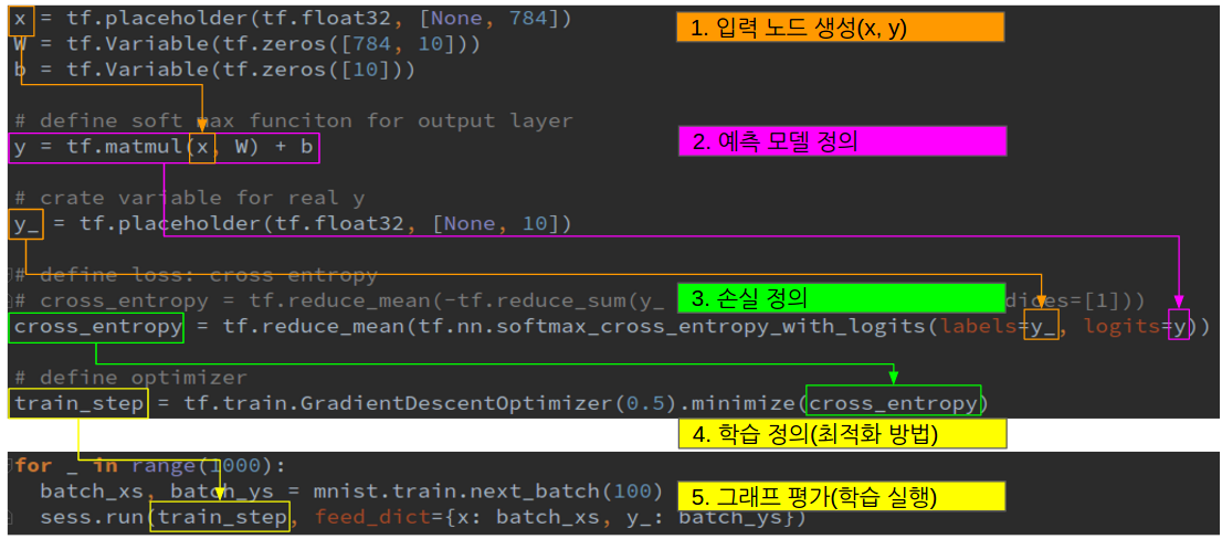
- 입력 노드를 생성
- 입력노드 x에 대한 모델의 출력값 y를 예측하는 모델을 정의
- 예측값 y와 실제값 y_를 이용하여 모델의 손실을 정의
- 모델의 손실을 이용하여 최적화 방법, 즉 학습을 정의
- 반복적으로 그래프를 평가하여 학습을 실행
이 글에서는 위와 동일한 그래프를 좀 더 객체지향적으로 구성하나, 기본 뼈대는 아래 그림과 같이 동일하다.
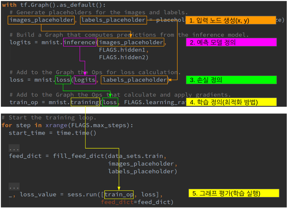
- 입력 노드 정의
- inference() 모델 정의하기
- loss() 손실 정의하기
- training() 최적화 방법 정의하기
이제 각각을 살펴본다. 그래프 정의는mechanics/mnist.py에 위치한다.
입력 노드
훈련 데이터셋의 입력/출력 값을 저장할 placeholder를 정의한다.
1 2 3 4 5 6 7 8 9 10 11 12 13 14# Generate placeholders for the images and labels. images_placeholder, labels_placeholder = placeholder_inputs(FLAGS.batch_size) ... def placeholder_inputs(batch_size): """Generate placeholder variables to represent the input tensors. Args: batch_size: The batch size will be baked into both placeholders. Returns: images_placeholder: Images placeholder. labels_placeholder: Labels placeholder. """ images_placeholder = tf.placeholder(tf.float32, shape=(batch_size, mnist.IMAGE_PIXELS)) labels_placeholder = tf.placeholder(tf.int32, shape=(batch_size)) return images_placeholder, labels_placeholder
image_placeholder의 shape의 경우 mnist.IMAGE_PIXELS을 파라미터로 받는다.
1 2 3# The MNIST images are always 28x28 pixels. IMAGE_SIZE = 28 IMAGE_PIXELS = IMAGE_SIZE * IMAGE_SIZE
inference()
mnist.inference()에서는 예측값을 계산할 모델을 정의한다.
1 2 3 4# Build a Graph that computes predictions from the inference model. logits = mnist.inference(images_placeholder, FLAGS.hidden1, FLAGS.hidden2)
여기에서 구성하려는 모델의 네트워크는 다음과 같다.
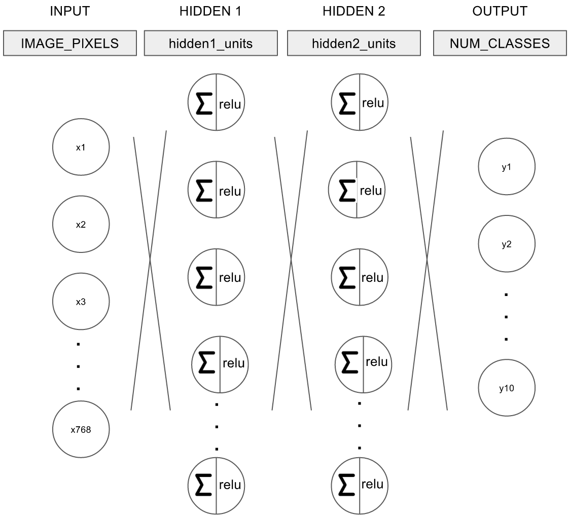
그림. MNIST 예제 네트워크
- 입력 입력은 IMAGE_PIXELS, 즉 768개의 노드로 구성
- 히든 레이어 1 1st 히든 레이어는 RELU를 활성화 함수로 사용
- 히든 레이어 2 2nd 히든 레이어는 RELU를 활성화 함수로 사용
- 출력 출력은 NUM_CLASSES, 즉 10개의 노드로 구성
첫 번째 히든 레이어를 구현한 코드는 다음과 같다.
1 2 3 4 5 6 7 8 9 10 11 12 13 14 15 16 17 18def inference(images, hidden1_units, hidden2_units): """Build the MNIST model up to where it may be used for inference. Args: images: Images placeholder, from inputs(). hidden1_units: Size of the first hidden layer. hidden2_units: Size of the second hidden layer. Returns: softmax_linear: Output tensor with the computed logits. """ # Hidden 1 with tf.name_scope('hidden1'): weights = tf.Variable( tf.truncated_normal([IMAGE_PIXELS, hidden1_units], stddev=1.0 / math.sqrt(float(IMAGE_PIXELS))), name='weights') biases = tf.Variable(tf.zeros([hidden1_units]), name='biases') hidden1 = tf.nn.relu(tf.matmul(images, weights) + biases)
파라미터 weights와 biases에 대한 변수를 선언하고, tf.matmul()을 통해 W * x + b를 계산한 후 tf.nn.relu() 활성화 함수를 통과시킨다. 두 번째 히든레이어와 출력 레이어도 비슷한 방법으로 구현한다.
1 2 3 4 5 6 7 8 9 10 11 12 13 14 15 16 17 18 19# Hidden 2 with tf.name_scope('hidden2'): weights = tf.Variable( tf.truncated_normal([hidden1_units, hidden2_units], stddev=1.0 / math.sqrt(float(hidden1_units))), name='weights') biases = tf.Variable(tf.zeros([hidden2_units]), name='biases') hidden2 = tf.nn.relu(tf.matmul(hidden1, weights) + biases) # Linear with tf.name_scope('softmax_linear'): weights = tf.Variable( tf.truncated_normal([hidden2_units, NUM_CLASSES], stddev=1.0 / math.sqrt(float(hidden2_units))), name='weights') biases = tf.Variable(tf.zeros([NUM_CLASSES]), name='biases') logits = tf.matmul(hidden2, weights) + biases return logits
loss()
모델의 예측값과 실제 레이블간의 차이, 즉 손실을 계산한다.
1 2# Add to the Graph the Ops for loss calculation. loss = mnist.loss(logits, labels_placeholder)
이때 logits와 labels_placeholder는 서로 다른 shape을 가진다.
1 2 3 4 5 6 7 8logits Out[2]: <tf.Tensor 'softmax_linear/add:0' shape=(100, 10) dtype=float32> labels_placeholder Out[3]: <tf.Tensor 'Placeholder_1:0' shape=(100,) dtype=int32> logits[1] Out[4]: <tf.Tensor 'strided_slice:0' shape=(10,) dtype=float32> labels_placeholder[1] Out[5]: <tf.Tensor 'strided_slice_1:0' shape=() dtype=int32>
모델의 예측값인 logits의 경우 shape이 (배치사이즈, 출력 레이블의 수)이지만, 실제 레이블은 shape이 (배치사이즈, 1) 다. 이는 MNIST 데이터셋을 one-hot 벡터 형태로 로드하지 않았기 때문이다. 손실 함수로는 크로스 엔트로피(cross entropy) 함수를 사용하며, 레이블의 shape을 one-hot 벡터로 변경하기 위해 sparse_softmax_cross_entropy_with_logits() 함수를 사용한다.
1 2 3 4 5 6 7 8 9 10 11 12def loss(logits, labels): """Calculates the loss from the logits and the labels. Args: logits: Logits tensor, float - [batch_size, NUM_CLASSES]. labels: Labels tensor, int32 - [batch_size]. Returns: loss: Loss tensor of type float. """ labels = tf.to_int64(labels) cross_entropy = tf.nn.sparse_softmax_cross_entropy_with_logits( labels=labels, logits=logits, name='xentropy') return tf.reduce_mean(cross_entropy, name='xentropy_mean')
참고로 getting_started/mnist_ml_step_by_step.py 예제에서는 MNIST 데이터셋을 one-hot 벡터로 로드했고, 이 경우에는 softmax_cross_entropy_with_logits() 함수를 손실함수로 사용했다.
1 2 3mnist = input_data.read_data_sets("MNIST_data/", one_hot=True) ... cross_entropy = tf.reduce_mean(tf.nn.softmax_cross_entropy_with_logits(labels=y_, logits=y))
training()
손실 함수를 이용하여 모델을 학습한다.
1 2# Add to the Graph the Ops that calculate and apply gradients. train_op = mnist.training(loss, FLAGS.learning_rate)
최적화함수로는 그래디언트 디센트(Gradient Descent)를 사용한다.
1 2 3 4 5 6 7 8 9 10 11 12 13 14 15 16 17 18 19 20def training(loss, learning_rate): """Sets up the training Ops. Creates a summarizer to track the loss over time in TensorBoard. Creates an optimizer and applies the gradients to all trainable variables. The Op returned by this function is what must be passed to the `sess.run()` call to cause the model to train. Args: loss: Loss tensor, from loss(). learning_rate: The learning rate to use for gradient descent. Returns: train_op: The Op for training. """ # Add a scalar summary for the snapshot loss. tf.summary.scalar('loss', loss) # Create the gradient descent optimizer with the given learning rate. optimizer = tf.train.GradientDescentOptimizer(learning_rate) # Use the optimizer to apply the gradients that minimize the loss # (and also increment the global step counter) as a single training step. train_op = optimizer.minimize(loss) return train_op
tf.summary.scalar()는 텐서보드에서 학습 과정을 시각화할 때 사용할 데이터를 직렬화하기 위한 메서드 중 하나다. 일단은 무시하고, 조금 후에 다룬다.
모델 학습하기
세션 생성 및 변수 초기화
데이터셋 로드되고 그래프가 모두 정의되면, 세션을 생성하고 변수(Variable)을 초기화하여 훈련을 시작할 준비를 한다.
1 2 3 4 5 6 7# Add the variable initializer Op. init = tf.global_variables_initializer() # Create a session for running Ops on the Graph. sess = tf.Session() # And then after everything is built: # Run the Op to initialize the variables. sess.run(init)
반복학습과 데이터 피드
모델을 반복적으로 훈련한다. 이때 훈련 데이터셋에서 배치 사이즈만큼의 데이터를 전달한다.
1 2 3 4 5 6 7 8 9 10 11 12 13 14 15 16 17 18 19def run_training(): ... # Start the training loop. start_time = time.time() for step in xrange(FLAGS.max_steps): feed_dict = fill_feed_dict(data_sets.train, images_placeholder, labels_placeholder) _, loss_value = sess.run([train_op, loss], feed_dict=feed_dict) ... def fill_feed_dict(data_set, images_pl, labels_pl): images_feed, labels_feed = data_set.next_batch(FLAGS.batch_size, FLAGS.fake_data) feed_dict = { images_pl: images_feed, labels_pl: labels_feed, } return feed_dict
피드된 실제 데이터는 다시 그래프를 거꾸로 가면서 입력 placeholder로 전달된다.
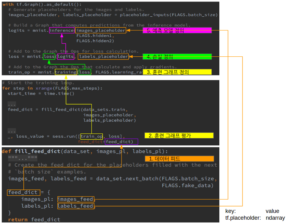
feed_dict의 키는 tf.placeholder이며, 값은 numpy.ndarray다. 세션을 실행하여 훈련 그래프를 평가하면, 아래와 같이 feed_dict_string에 key:value형태로 저장된다.
1 2 3 4 5 6 7 8 9 10 11 12# Validate and process feed_dict. if feed_dict: for feed, feed_val in feed_dict.items(): for subfeed, subfeed_val in _feed_fn(feed, feed_val): try: subfeed_t = self.graph.as_graph_element(subfeed, allow_tensor=True, allow_operation=False) np_val = np.asarray(subfeed_val, dtype=subfeed_dtype) subfeed_name = compat.as_bytes(subfeed_t.name) feed_dict_string[subfeed_name] = np_val # Create a fetch handler to take care of the structure of fetches. fetch_handler = _FetchHandler(self._graph, fetches, feed_dict_string)
그리고 placeholder로 선언된 변수(입력, 출력)에 실제 ndarray값이 할당되고 그래프가 평가된다.
학습 상태 확인
학습이 제대로 되고 있는지 확인하기 위해, 매 100 스텝마다 훈련 에러를 출력한다.
1 2 3 4 5 6# Write the summaries and print an overview fairly often. if step % 100 == 0: # Print status to stdout. duration = time.time() - start_time print('Step %d: loss = %.2f (%.3f sec)' % (step, loss_value, duration)) start_time = time.time()
모델 평가하기
학습된 모델이 과적합이 발생하지 않았는지 모델을 평가하는 과정이 필요하다. 이 글에서는 별도로 설명하지 않는다. 자세한 내용은 TensorFlow Mechanics 101의 "Evaluate the Model"을 참고한다.
tf.contrib.learn를 사용한 IRIS 예제
텐서보드를 보기 전에 예제 하나를 더 살펴 본다. 이 장에서는 tf.contrib.learn Quickstart에서 설명하는 내용을 차례차례 따라해 본다. 텐서플로우의 고수준 API인 tf.contrib.learn을 사용하여 IRIS 꽃 분류 예제를 구현한다. 고수준 API를 사용하면 모델을 정의하고 평가하는 일이 훨씬 간편해진다. 나중에 텐서보드를 사용할 때도 마찬가지다. 저수준 API를 사용하는 경우 훈련 과정을 시각화할 메트릭을 일일이 지정해야 한다. 반면 tf.contrib.learn에서 제공하는 Monitor API를 사용하면 손쉽게 메트릭를 선언하여 사용할 수 있다. 이 장의 예제 코드는 tensorboard/iris_ml_step_by_step_contrib.py에 위치한다.
IRIS 분류 문제 정의
IRIS 꽃 분류 문제의 경우 입력 변수는 꽃받침 길이(sepal length), 꽃받침 너비(sepal width), 꽃잎 길이(petal length), 꽃잎 너비(petal width)다. 출력 변수는 IRIS의 세 품종인 세토사(Setosa), 버시컬러(Versicolour), 버지니카(Virginica) 중 하나다. IRIS 꽃 분류 문제에서는 IRIS 꽃 품종별로 관측된 {입력:출력} 데이터셋을 학습한 후, 임의의 IRIS 꽃의 입력값에 대해 해당 꽃이 IRIS의 세가지 품종 중 어떤 품종인지 구분하는 문제다.
학습 데이터셋 탐색하기
IRIS 데이터셋 파일은 예제 프로젝트의 tensorboard/에 위치하며 훈련 데이터셋은 iris_training.csv, 테스트 데이터셋은 iris_test.csv 파일이다. 각 파일은 아래와 같은 형태를 가진다.
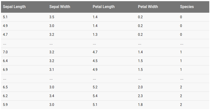
그림. IRIS 데이터셋 파일 폼새
학습하기
tf.contrib.learn API를 사용하여 IRIS 분류 모델을 훈련한다. tf.contrib.learn API를 사용하더라도 저수준 API를 사용하여 훈련하는 것과 동일한 프로세스를 따른다.
데이터셋 로드하기
학습 데이터셋을 로드한다. 훈련 데이터셋과 테스트 데이터셋을 각각 로드한다. 특성 값(입력값)은 float32으로, 타겟 값(출력값)은 int로 타입을 지정한다.
1 2 3 4 5 6 7 8 9# Load datasets. training_set = tf.contrib.learn.datasets.base.load_csv_with_header( filename=IRIS_TRAINING, target_dtype=np.int, features_dtype=np.float32) test_set = tf.contrib.learn.datasets.base.load_csv_with_header( filename=IRIS_TEST, target_dtype=np.int, features_dtype=np.float32)
입력 노드 생성하기
모델의 입력 값의 특성을 정의한다. 입력값은 실수이며, 4개의 차원을 가진다.
1feature_columns = [tf.contrib.layers.real_valued_column("", dimension=4)]
예측 모델 정의하기
모델을 정의한다. 학습 모델을 정의하기 위해서는 아래의 3가지 요소를 정의해야 한다.
- 네트워크 그래프
- 손실
- 최적화 함수
이 예제는 멀티클래스 분류 모델이며, 이 경우 DNNClassifier를 사용한다. 아래 코드를 보자.
1 2 3 4 5# Build 3 layer DNN with 10, 20, 10 units respectively. classifier = tf.contrib.learn.DNNClassifier(feature_columns=feature_columns, hidden_units=[10, 20, 10], n_classes=3, model_dir="/tmp/iris_model")
- 입력 레이어 입력 레이어는 이전에 선언한 feature_columns를 전달
- 히든 레이어 총 3개의 히든 레이어를 가지며, 각각 10개, 20개, 10개의 노드를 가진다
- 출력 레이어 출력 레이어에는 분류하려는 레이블의 수, 3개의 노드를 가진다.
DNNClassifier는 이외에도 여러가지 인자를 받을 수 있으며, 최적화 함수의 경우 "optimizer"를 이용하여 전달할 수 있다. 기본값은 Adagrad다.
1 2"""optimizer: An instance of `tf.Optimizer` used to train the model. If `None`, will use an Adagrad optimizer."""
손실의 경우 별도로 전달받지 않으며 멀티클래스 분류 모델에서 일반적으로 사용하는 softamx cross entropy를 손실 함수로 내부적으로 사용한다. 아래는 해당 tf.contrib.learn 패키지의 관련 주석문이다.
1 2 3 4 5 6 7 8 9def _multi_class_head(n_classes, label_name=None, weight_column_name=None, enable_centered_bias=False, head_name=None, thresholds=None, metric_class_ids=None): """Creates a _Head for multi class single label classification. The Head uses softmax cross entropy loss."""
훈련하기
정의된 모델에 대해 훈련 데이터셋을 이용하여 반복적으로 훈련시킨다.
1 2 3 4 5 6# Define the training inputs def get_train_inputs(): x = tf.constant(training_set.data) y = tf.constant(training_set.target) ... classifier.fit(input_fn=get_train_inputs, steps=2000)
fit() 함수는 이외에도 batch_size와 monitors를 전달할 수 있다. batch_size는 미니배치 사이즈이며, monistors는 로깅하거나 텐서보드를 통해 시각화할 메트릭을 정의한다.
평가하기
테스트셋을 이용하여 훈련된 모델을 평가한다. 그리고 결과값에서 정확도(accuracy)를 출력한다.
1 2 3 4 5 6 7 8 9# Define the test inputs def get_test_inputs(): x = tf.constant(test_set.data) y = tf.constant(test_set.target) return x, y ... # Evaluate accuracy. eval_result = classifier.evaluate(input_fn=get_test_inputs, steps=1) accuracy_score = eval_result["accuracy"]
참고로 리턴된 eval_result 전체 데이터는 다음과 같다.
1 2 3 4 5 6eval_result Out[2]: {'accuracy': 0.96666664, 'auc': 0.97500002, 'global_step': 48000, 'loss': 0.72319746}
텐서보드(TensorBoard) 사용하기
지금까지 다룬 예제를 이용하여 텐서보드를 사용하는 방법을 설명한다. 이 장에서는 TensorBoard: Visualizing Learning에서 설명하는 내용을 다룬다.
간단한 예제
먼저 간단한 예제를 통해 텐서보드가 동작하는 방식을 살펴보자. 이 절의 예제는 지난 글에서 다룬 getting_started/mnist_ml_step_by_step.py에 summary 오퍼레이션을 추가한 예제로, tensorboard/mnist_ml_step_by_step_vis.py에 위치한다.
summary 오퍼레이션 추가하기
예를 들어 훈련 에폭이 진행될 때마다 손실이 줄어드는지 확인하고 싶다고 하자. 이 경우 측정하려는 오퍼레이션에 대해 tf.summary 오퍼레이션을 추가한다. 손실의 경우 스칼라 값이므로, tf.summary.scalar를 이용한다. tf.summary 오퍼레이션을 등록할 때 첫번째 파라미터로 오퍼레이션을 식별할 수 있는 태그를 전달한다.
1 2 3 4 5# define loss: cross entropy # cross_entropy = tf.reduce_mean(-tf.reduce_sum(y_ * tf.log(y), reduction_indices=[1])) cross_entropy = tf.reduce_mean(tf.nn.softmax_cross_entropy_with_logits(labels=y_, logits=y)) # summary scalar for loss tf.summary.scalar('cross_entropy', cross_entropy)
그래프로 시각화하면 다음과 같다.
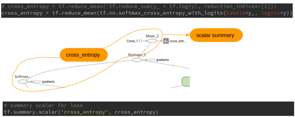
그림. cross_entropy 오퍼레이션에 tf.summary.scalar 오피레이션을 연결
Summary Operations에서 제공하는 오퍼레이션의 종류는 다음과 같다.
- tensor_summary
- scalar
- histogram
- image
가중치 W에 대해서는 평균, 표준편차, 최대값, 최소값을 각각 추가하자.
1 2 3 4 5 6 7# summary scalar for W mean = tf.reduce_mean(W) stddev = tf.sqrt(tf.reduce_mean(tf.square(W - mean))) tf.summary.scalar('mean', mean) tf.summary.scalar('stddev', stddev) tf.summary.scalar('max', tf.reduce_max(W)) tf.summary.scalar('min', tf.reduce_min(W))
특히 가중치의 경우 분포를 보면 도움이 되므로, 히스트그램 오퍼레이션도 추가한다.
1 2# summary histogram for W tf.summary.histogram('histogram', W)
입력의 경우 이미지이므로 tf.summary.image를 사용한다. 아래는 입력 이미지 중에서 최대 10개의 이미지를 출력한다.
1 2 3# summary image for x image_shaped_input = tf.reshape(x, [-1, 28, 28, 1]) tf.summary.image('input', image_shaped_input, 10)
summary 오퍼레이션 병합하기
추가된 summary 오퍼레이션은 모델 그래프와는 별개로 평가해야 하며, 개별 오퍼레이션 각각을 평가해야 한다. 쉽게 평가하기 위해 summary 오퍼레이션을 하나의 오퍼레이션으로 병합한다.
1 2# merge all summary ops into a single op merged = tf.summary.merge_all()
파일로 저장하기
텐서보드는 각 summary 오퍼레이션이 평가된 결과가 저장된 파일을 기반으로 한다. 이를 위해 파일에 저장할 수 있는 FileWriter를 생성한다. 이때 이벤트 파일이 생성될 디렉토리 위치와, 추가로 텐서보드에 그래프를 표시하기 위해 그래프도 파라미터로 전달한다.
1 2# write summary to disk for TensorBoard visualization train_writer = tf.summary.FileWriter('/home/itrocks/Downloads/train', sess.graph)
평가하기
세션을 통해 그래프와 summary 오퍼레이션들을 평가한다. 그리고 평가된 summary를 파일로 저장한다.
1 2 3 4 5 6 7for i in range(2000): batch_xs, batch_ys = mnist.train.next_batch(100) # run summary op and train op summary, _ = sess.run([merged, train_step], feed_dict={x: batch_xs, y_: batch_ys}) # write summary events to disk train_writer.add_summary(summary, i) train_writer.close()
학습이 끝나면 FileWriter에 파라미터로 전달한 디렉토리에 이벤트 파일이 생성된다.
1 2 3 4 5 6 7$ pwd /home/itrocks/Downloads/train $ ls -al total 17144 drwxrwxr-x 2 itrocks itrocks 4096 Mar 27 16:40 . drwxr-xr-x 3 itrocks itrocks 20480 Mar 27 10:43 .. -rw-rw-r-- 1 itrocks itrocks 17523134 Mar 27 16:40 events.out.tfevents.1490600444.aidentify
텐서보드 실행하기
텐서보드는 웹 기반이며, 실행할 때 이벤트 파일이 생성된 디렉토리를 파라미터로 전달한다.
1 2 3 4 5 6 7 8$ tensorboard --logdir=/home/itrocks/Downloads/train I tensorflow/stream_executor/dso_loader.cc:135] successfully opened CUDA library libcublas.so.8.0 locally I tensorflow/stream_executor/dso_loader.cc:135] successfully opened CUDA library libcudnn.so.5 locally I tensorflow/stream_executor/dso_loader.cc:135] successfully opened CUDA library libcufft.so.8.0 locally I tensorflow/stream_executor/dso_loader.cc:135] successfully opened CUDA library libcuda.so.1 locally I tensorflow/stream_executor/dso_loader.cc:135] successfully opened CUDA library libcurand.so.8.0 locally Starting TensorBoard 41 on port 6006 (You can navigate to http://127.0.1.1:6006)
텐서보드(http://localhost:6006)로 접속한다.
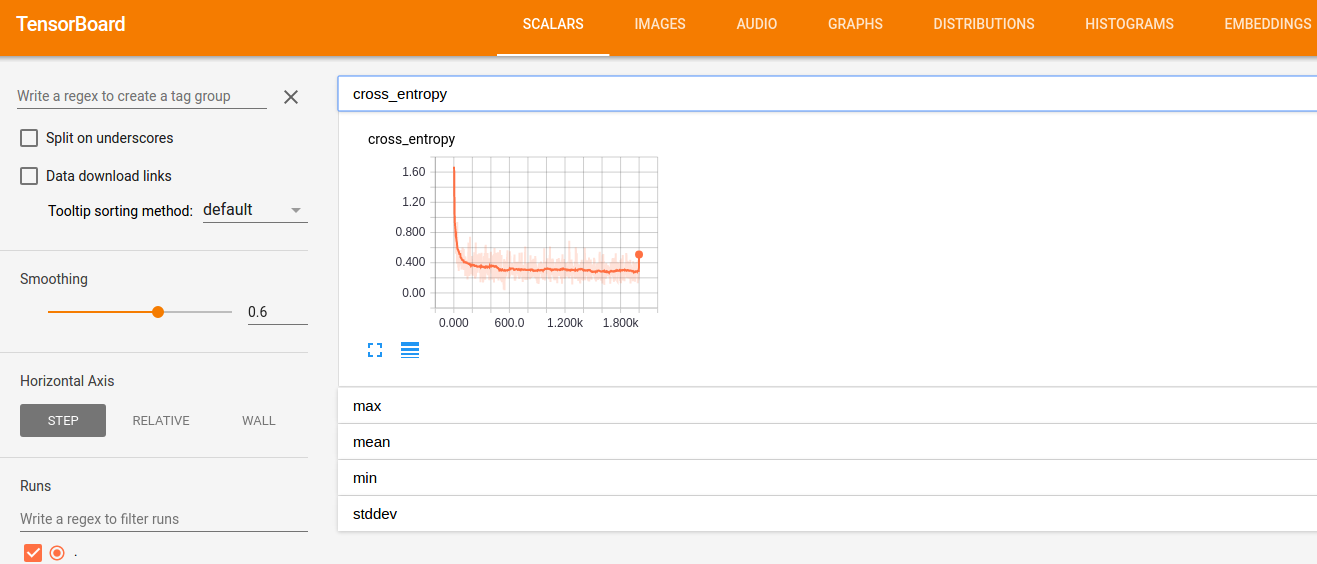
그림. 텐서보드 접속화면
tf.summary 유형별로 메뉴가 있으며(SCALARS, IMAGES, HISTOGRAM, 등), 각 화면에는 tf.summary로 추가한 메트릭을 태그 이름을 클릭하여 확인할 수 있다.
tf.contrib.learn을 이용한 로깅과 텐서보드 사용하기
tf.contrib.learn 고수준 API를 사용하면 훈련과정에 대한 상세한 로깅을 출력하거나, 파일로 생성하여 텐서보드에서 쉽게 시각화할 수 있다. 이 장에서는 Logging and Monitoring Basics with tf.contrib.learn에서 설명하는 내용을 다룬다. 이 장에서 다루는 예제는 IRIS 예제인 tensorboard/iris_ml_step_by_step_contrib.py을 확장한 것으로, tensorboard/iris_ml_step_by_step_contrib_mon.py에 위치한다.
로깅 레벨 설정하기
텐서플로우의 로깅 레벨 정책은 DEBUG > INFO > WARN > ERROR > FATAL이며, 기본 로깅 레벨은 WARN이다. 모델을 만들어가는 과정에는 INFO 레벨을 사용하여 학습 과정을 살펴보는게 좋다. import 구문 바로 아래에 로깅 레벨을 변경할 수 있도록 설정한다.
1 2# set logging level to INFO (default: WARN) tf.logging.set_verbosity(tf.logging.INFO)
실행하면 아래와 같이 100스텝마다 훈련 에러를 INFO 로그로 확인할 수 있다.
1 2 3 4INFO:tensorflow:Saving checkpoints for 1 into /tmp/iris_model/model.ckpt. INFO:tensorflow:loss = 1.16283, step = 1 INFO:tensorflow:global_step/sec: 1072.63 INFO:tensorflow:loss = 0.19813, step = 101
모니터링 API
tf.contib.learn은 모니터링을 위한 API를 제공하며 종류는 아래와 같다.
| Monitor | 설명 |
| CaptureVariable | 매 n 훈련 스텝마다 변수의 값을 저장한다 |
| PrintTensor | 매 n 훈련 스텝마다 텐서의 값을 로그로 남긴다 |
| ValiationMonitor | 매 n 훈련 스텝마다 설정된 평가 메트릭을 로그로 남긴다.
또한 특정 조건을 만족하면 early stopping할 수 있는 기능도 제공한다 |
이 글에서는 ValidationMonitor를 이용하여 훈련 단계에 테스트 데이터셋을 이용하여 평가를 병행하는 방법과, MetricSpec을 이용하여 커스텀 메트릭을 만드는 방법을 소개한다.
스트리밍 평가(streaming evaluation)
스트리밍 평가란 훈련 단계에 평가를 동시에 진행하는 것으로, 과적합이 발생하는지 모니터링하기 위해 사용한다. 아래와 같이 테스트 데이터셋을 인자로 전달하여 ValidationMonitor를 생성한다.
1 2 3 4 5# Validation Monitor for evaluation at every 50 training steps validation_monitor = tf.contrib.learn.monitors.ValidationMonitor( test_set.data, test_set.target, every_n_steps=50)
ValidationMonitor는 훈련 단계에 생성된 체크포인트 모델파일을 기반으로 평가를 실행한다. 체크포인트 파일 생성 기준은 600초가 기본값이다. IRIS 예제의 경우 수초 이내에 학습이 완료되므로, 체크포인트 파일이 생성되는 기준을 1초로 변경하여 매초마다 체크포인트가 생성될 수 있도록 한다.
1 2 3 4 5 6 7# Build 3 layer DNN with 10, 20, 10 units respectively. classifier = tf.contrib.learn.DNNClassifier( feature_columns=feature_columns, hidden_units=[10, 20, 10], n_classes=3, model_dir="/tmp/iris_model", config=tf.contrib.learn.RunConfig(save_checkpoints_secs=1))
** 참고 **
model_dir에 저장된 체크포인트 모델은 삭제되지 않으며 유지된다. 따라서 매번 훈련을 실행하는 경우 이전에 저장된 모델 파일을 기반으로 추가로 학습이 진행된다. 예를 들어 이 예제를 2번 실행하는 경우 각각 2000스텝이 실행되어, 최종적으로는 4000번 스텝이 실행된 모델이 생성된다. 처음부터 새로 모델을 학습하려면 model_dir에 있는 파일을 모두 삭제한다.
생성한 ValidationMonitor를 모델을 학습할 때 monitors 인자로 전달한다.
1 2 3 4# Fit model. classifier.fit(input_fn=get_train_inputs, steps=2000, monitors=[validation_monitor])
훈련을 실행하면, 아래와 같이 Validation 결과도 INFO 로그로 출력되는 것을 확인할 수 있다.
1 2 3INFO:tensorflow:Validation (step 2651): loss = 0.104998, auc = 0.998333, global_step = 2602, accuracy = 0.966667 INFO:tensorflow:global_step/sec: 106.355 INFO:tensorflow:loss = 0.0352977, step = 2701
MetricSpec: 커스텀 메트릭 만들기
ValidationMonitor의 평가 메트릭은 기본적으로 loss, auc, accuracy를 포함한다. 추가로 메트릭을 만들고 싶으면 MetricSpec을 사용한다. 먼저 precision과 recall에 대한 메트릭을 정의한다.
1 2 3 4 5 6 7 8 9 10 11# define custom metric validation_metrics = { "precision": tf.contrib.learn.MetricSpec( metric_fn=tf.contrib.metrics.streaming_precision, prediction_key=tf.contrib.learn.PredictionKey.CLASSES), "recall": tf.contrib.learn.MetricSpec( metric_fn=tf.contrib.metrics.streaming_recall, prediction_key=tf.contrib.learn.PredictionKey.CLASSES) }
- metric_fn 메트릭 값을 리턴할 함수 tf.contrib.metrics.streaming_precision과 같이 미리 정의된 함수를 사용하거나, 커스텀 메트릭 함수를 정의할 수도 있다
- predictoin_key 모델에서 리턴한 예측값을 나타내는 텐서에 대한 키 DNNClassifier 모델에서는 tf.contrib.learn.PredictionKey.CLASSES를 키로 리턴한다
정의한 커스텀 메트릭을 ValidationMonitor에 아래와 같이 추가한다.
1 2 3 4 5validation_monitor = tf.contrib.learn.monitors.ValidationMonitor( test_set.data, test_set.target, every_n_steps=50, metrics=validation_metrics)
학습을 실행하면 아래와 같이 추가한 precision과 recall 메트릭도Validation 결과에 추가되어 로깅되는 것을 확인할 수 있다.
1INFO:tensorflow:Validation (step 700): loss = 0.0531897, auc = 0.998333, global_step = 657, recall = 1.0, precision = 1.0, accuracy = 0.966667
텐서보드로 시각화하기
ValidationMonitor가 생성한 로그를 텐서보드로 시각화한다. 먼저 텐서보드를 실행한다. 실행할 때 모델을 저장할 디렉토리(model_dir)을 인자로 전달한다.
1 2 3 4 5 6 7 8$ tensorboard --logdir=/tmp/iris_model/ I tensorflow/stream_executor/dso_loader.cc:135] successfully opened CUDA library libcublas.so.8.0 locally I tensorflow/stream_executor/dso_loader.cc:135] successfully opened CUDA library libcudnn.so.5 locally I tensorflow/stream_executor/dso_loader.cc:135] successfully opened CUDA library libcufft.so.8.0 locally I tensorflow/stream_executor/dso_loader.cc:135] successfully opened CUDA library libcuda.so.1 locally I tensorflow/stream_executor/dso_loader.cc:135] successfully opened CUDA library libcurand.so.8.0 locally Starting TensorBoard 41 on port 6006 (You can navigate to http://127.0.1.1:6006)
텐서보드로 접속(http://localhost:6006)하면 시각화된 메트릭을 확인할 수 있다.
학습 메트릭 살펴보기
학습 과정에서 주요하게 모니터링해야할 메트릭은 다음과 같으며, CS231n: Convolutional Neural Networks for Visual Recognition: Neural Networks Part 3: Learning and Evaluation을 참고했다.
손실 함수
에폭이 진행될수록 손실 함수가 감소하느지, 그리고 감소하는 형태를 확인한다.
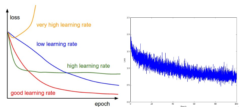
그림. 손실과 학습률의 관계(왼쪽)와 손실의 추이
(출처: CS231n Part 3: Learning and Evaluation)
왼쪽 그림에서 학습률과 손실의 추이간의 관계는 다음과 같다.
- 학습률이 낮을 경우(파란색) 학습이 선형적으로 진행
- 학습률이 조금 높을 경우(녹색) 초반에는 기하급수적으로 손실이 감소하는 것처럼 보이나, 어느정도 지나면 학습이 진행되지 않음
- 학습률이 많이 높을 경우(노란색) 학습이 안됨
따라서, 학습이 진행되면서 손실의 추세를 보고 학습률을 조정한다.
오른쪽 그림의 경우 손실은 선형보다는 빠르게 줄어든다. 다만 손실의 변동폭이 큰데, 이는 미니배치의 크기가 작기 때문일수 있다. 아래는 위의 IRIS 예제에서 시각화한 손실율이다.
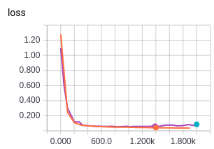
그림. IRIS 예제의 손실
정확도
정확도(accuracy)는 훈련 정확도와 평가 정확도를 함께 관찰한다. 훈련 정확도(training accuracy)와 평가 정확도(validation accuracy)간의 차이가 과적합(overfitting)된 정도다.
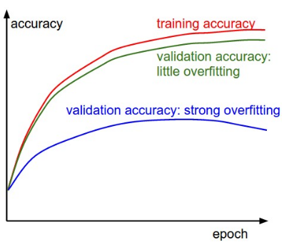
그림. 훈련 정확도와 평가 정확도
(출처: CS231n Part 3: Learning and Evaluation)
- 차이가 큰 경우(파란색) 과적합이 크게 발생한 경우로, 데이터 regularizaton을 적용하거나 더 많은 데이터셋으로 훈련/평가를 시도한다
- 차이가 없는 경우(녹색) 평가 정확도가 훈련 정확도를 잘 쫓아가는 경우로, 네트워크 사이즈(노드 개수, 레이어 개수)를 키우면서 훈련/평가를 시도한다
아래는 위의 IRIS 예제에서 시각화한 평가 정확도다. 텐서보드에서 훈련 메트릭과 평가 메트릭을 동시에 볼 수 있는 차트가 있는지는 확인하지 못했다.
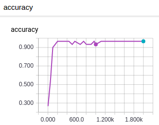
그림. IRIS 예제의 평가 정확도
weight:update 비율
마지막으로 주요하게 관찰할 메트릭은 weight:update 비율(네트워크 전체, 레이어별)로, weight의 크기에 비해 변경되는 가중치의 update 크기간의 비율이다. 아래와 같이 계산할 수 있다.
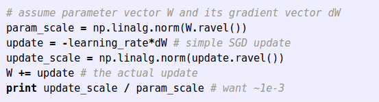
그림. weight:update ratio 계산
(출처: CS231n Part 3: Learning and Evaluation)
대체로 1e-3(0.001) 정도의 값을 가지는게 좋다고 한다. 아래는 Deeplearning4J의 시각화 도구에서 제공하는 weight:update 비율에 대한 시각화로, 학습이 진행되면서 log(-3) = 0.001로 근사하는 것을 확인할 수 있다.
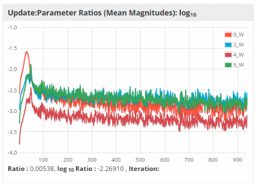
그림. 에폭별 weight:update ratio 추세
(출처: Visualize, Monitor and Debug Network Learning)
텐서보드에서 weight:update 비율에 대한 메트릭을 tb.contrib.learn에서 제공하지는 않는 듯하다.
다음 여정으로
이 정도면 텐서플로우로 구현된 코드를 읽을 수 있을 정도는 된 듯하다. 다음에는 원래 목표였는 GAN에 대해서 소개할 수 있도록 하겠다.
참고자료
- 텐서플로우(TensorFlow) 시작하기
- TensorFlow Mechanics 101
- StartingTensorFlow
- tf.contrib.learn Quickstart
- TensorBoard: Visualizing Learning
- Summary Operations
- Logging and Monitoring Basics with tf.contrib.learn
- Visualize, Monitor and Debug Network Learning
- CS231n: Convolutional Neural Networks for Visual Recognition: Neural Networks Part 3: Learning and Evaluation
Portions of this page are modifications based on work created and shared by Google and used according to terms described in the Creative Commons 3.0 Attribution License.