TF-Slim 시작하기

TF-Slim은 저수준의 텐서플로우 API를 간편하게 사용할 수 있는 고수준 경량 API로써, 텐서플로우 저수준 API를 사용하여 모델을 정의, 학습, 평가하는 과정을 간소화한다. 특히 이미지를 분류하는 작업의 경우, 성능이 검증된 다양한 이미지 모델(VGG, Inception, ResNet 등)에 대해 이미지넷 데이터셋을 기반으로pre-trained된 모델을 기반으로 fine-tuning하는 과정이 단순화되어 있다. 이 글에서는 TF-Slim에 대한 개념을 설명하고 이를 MNIST 필기체 인식 문제를 해결해 본다. 그리고 스탠포드 대학교에서 제공하는 개 품종 이미지 데이터(Standford Dogs Dataset)를 이용하여 개를 분류하는 모델을 학습하고 평가하는 방법을 소개한다.
이 글은 TensorFlow-Slim과 TensorFlow-Slim image classification library을 참조했으며, 참조 글에서 제공하는 예제를 실제로 동작하도록 하는데 초점을 맞췄다. 개념적인 설명보다는 구현하는 코드를 먼저 보려면 TF-Slim Walkthrough가 도움이 된다.
장점
TF-Slim 라이브러리를 사용하면 텐서플로우를 사용하여 변수를 정의하고 오퍼레이션을 구성할 때 반복적으로 "복사-붙여넣기"하게 되는 코드간의 중복을 제거할 수 있다. 이를 통해 네트워크 모델을 더 적은 코드로 정의할 수 있고, 가독성이 높아지며 "복사-붙여넣기"할 때 저지르는 실수를 방지할 수 있다. 그리고 반복적인 기반 코드를 작성하는 과정보다 훈련하고 평가하는 과정에 더 충실할 수 있게 된다.
TF-Slim에서 제공하는 컴포넌트와 장점은 다음과 같다. 각 컴포넌트에 대한 자세한 설명은 다음 장에 설명한다.
스코프
텐서플로우에서는 변수의 이름을 한정하기 위해 tf.name_scope와 tf.variable_scope를 제공한다. 또한 TF-Slim에서는 중복되는 코드를 제거하기 위한 slim.arg_scope를 제공한다. slim.arg_scope를 사용하면 오퍼레이션마다 중복되는 인자값들을 공통화할 수 있어 코드가 간소화된다.
변수
변수를 생성하고 조작하는 방법을 단순화했다. 또한 모델 변수(slim.model_variable)라는 개념을 추가했다. 텐서플로우에서 변수는 훈련을 통해 업데이트하는 모델의 파라미터를 구성하는 변수(가중치, 바이어스 등)와, 훈련과정에는 필요하지만 모델을 구성하지 않는 일반 변수(global_step 등)로 구분할 수 있지만 프로그램 구문적으로는 구분되어 있지 않다. TF-Slim에서는 slim.model_variable 구문을 추가했으며, 모델 변수와 일반 변수를 프로그램 구문적으로구분할 수 있다.
레이어
가중치와 바이어스 등의 변수와 tf.nn.conv2d 등 오퍼레이션 관점이 아닌 추상화된 레이어 관점에서 모델을 구성할 수 있도록 레이어 함수가 추가되었다. 주요 레이어와 TF-Slim 레이어 함수는 다음과 같다.
| 레이어 | TF-Slim |
| BiasAdd | slim.bias_add |
| BatchNorm | slim.batch_norm |
| Conv2d | slim.conv2d |
| Conv2dInPlane | slim.conv2d_in_plane |
| Conv2dTranspose (Deconv) | slim.conv2d_transpose |
| FullyConnected | slim.fully_connected |
| AvgPool2D | slim.avg_pool2d |
| Dropout | slim.dropout |
| Flatten | slim.flatten |
| MaxPool2D | slim.max_pool2d |
| OneHotEncoding | slim.one_hot_encoding |
| SeparableConv2 | slim.separable_conv2d |
| UnitNorm | slim.unit_norm |
데이터
텐서플로우를 사용할 때 가장 까다로운 부분이 훈련/평가에 사용할 데이터셋 이터레이터를 구성하는 일이다. TF-Slim에서는 TFRecord 포맷을 기반으로 데이터셋(slim.dataset.Dataset)을 생성하고, 훈련/평가할 때 데이터를 피드해주는 데이터 프로바이더(slim.dataset_data_provider.DatasetDataProvider)를 추가하는 등을 과정이 텐서플로우보다는 간단히 구성할 수 있다.
손실 함수
자주 쓰이는 손실 함수에 대한 slim.losses 모듈을 제공한다. 텐서플로우에서도 손실 함수는 단순했기에 크게 차이는 없다. 다먼 멀티태스크 작업에서 여러개의 손실함수를 사용해야 하는 경우, 여러개의 손실 함수를 손쉽게 하나로 합칠 수 있다. 해 본적이 없어 이 글에서는 설명하지 않는다. 옵티마이저(optimizer)는 텐서플로우 옵티마이저를 그대로 사용한다.
훈련
반복적으로 훈련하기 위한 slim.learning 모듈을 제공한다. 텐서플로우에서도 데이터를 피드해주는 과정만 제외하면 훈련 과정 자체는 단순하므로 크게 차이는 없다.
평가
학습된 모델에 대한 평가를 위한 slim.evaluation 모듈을 제공한다.
메트릭
정확도, 재현율 등 자주 사용하는 메트릭을 쉽게 사용할 수 있는 slim.metrics 모듈을 제공한다.
네트워크
자주 사용하는 이미지 모델(VGG, Incetion, ResNet 등)을 쉽게 활용할 수 있도록 slim.nets 모듈을 제공한다. 예를 들어 기본 네트워크 모델로 VGG 모델을 사용하하는 경우 아래와 같이 모델을 임포트할 수 있다.
1 2import tensorflow.contrib.slim.nets vgg = tf.contrib.slim.nets.vgg
TF-Slim은 이러한 모델별로 이미지넷을 기반으로 학습한 체크포인트 파일을 제공한다. TF-Slim의 가장 큰 강점은 이러한 모델과 학습된 체크포인트 파일을 이용하여 자신의 태스크에 맞게 fine-tuning하는 과정이 단순하다는 점이다. 이미지넷을 기반으로 학습된 이미지 모델별 체크포인트 파일 목록은TensorFlow-Slim image classification library에서 확인할 수 있다.
예제 코드
이제 앞에서 설명한 TF-Slim 모듈을 예제를 바탕으로 좀 더 자세히 설명한다. 설명하는 순서와 사용하는 예제는 다음과 같다.
- 모델 정의
- 예제: MNIST 필기체 인식
- 데이터셋 준비
- 예제: MNIST필기체 인식
- 훈련
- 예제: MNIST필기체 인식
- fine-tuning
- 예제: 개 품종 분류
- 평가
- 예제: 개 품종 분류
전반적인 설명과 MNIST 예제는 tf-slim-tutorial에서, 개 품종 분류 예제는 dog-breed-classification.tf에서 클론할 수 있다.
1 2$ git clone https://github.com/socurites/tf-slim-tutorial.git $ git clone https://github.com/socurites/dog-breed-classification.tf.git
모델 정의하기
네트워크 모델을 정의하려면 변수, 오퍼레이션, 스코프(scope)가 필요하다. TF-Slim에서는 변수를 생성하는 방법이 간소화되었고, slim.arg_scope를 사용하여 오퍼레이션마다 중복되는 인자들을 공통화할 수 있다. 그리고 모델을 구성하는 레이어의 경우 변수가 아닌 추상화된 TF-Slim 레이어 함수를 사용하면 좀 더 쉽게 정의할 수 있다.
변수
native TF에서 변수를 생성, 초기화, 저장, 로드하는 방법
(예제: c01_defining_models/s01_variables/native_tf_variables.py)
텐서플로우와 TF-Slim에서 변수를 사용하는 방법을 비교하기 위해 native TF에서 어떻게 변수를 생성하고 사용하는지 살펴보자. 이 절의 내용은 TensorFlow > Programmer's Guide > Variables: Creation, Initialization, Saving, and Loading을 참고했다.
텐서플로우에서 변수를 생성하는 방법에는 3가지 종류가 있다.
- 미리 정해진 상수(constant)로 변수를 생성
- tf.zeros
- tf.ones
- 초기화 메커니즘에 따라 변수를 생성
- 시퀀스 텐서
- tf.linspace
- tf.range
- 랜덤 텐서
- tf.random_normal
- tf.truncated_normal
- 시퀀스 텐서
1 2 3 4 5 6 7bias_1 = tf.Variable(tf.zeros(shape=[200]), name="b1") weight_1 = tf.Variable(tf.lin_space(start=0.0, stop=12.0, num=3), name="w1") weight_2 = tf.Variable(tf.range(start=0.0, limit=12.0, delta=3), name="w2") weight_3 = tf.Variable(tf.random_normal(shape=[784, 200], mean=1.5, stddev=0.35), name="w3") weight_4 = tf.Variable(tf.truncated_normal(shape=[784, 200], mean=1.5, stddev=0.35), name="w4") print(weight_1) # >> Tensor("w1/read:0", shape=(3,), dtype=float32)
생성된 텐서 변수는 초기화한 후, 세션에서 실행하여 변수를 평가하여 값을 할당할 수 있다.
1 2 3 4 5 6 7 8 9 10 11 12 13 14 15 16 17 18 19 20 21 22 23 24 25with tf.Session() as sess: sess.run(init_op) val_b1 = sess.run(bias_1) val_w1, val_w2, val_w3, val_w4 = sess.run([weight_1, weight_2, weight_3, weight_4]) print(type(val_b1)) # >> <type 'numpy.ndarray'> print(val_w1.shape) # >> (3,) # 그래프로 변수 확인하기 plt.subplot(221) plt.hist(val_w1) plt.title('val_w1_linspace') plt.grid(True) plt.subplot(222) plt.hist(val_w2) plt.title('val_w2_range') plt.grid(True) plt.subplot(223) plt.hist(val_w3) plt.title('val_w3_random_normal') plt.grid(True) plt.subplot(224) plt.hist(val_w4) plt.title('val_w2_truncated_normal') plt.grid(True)
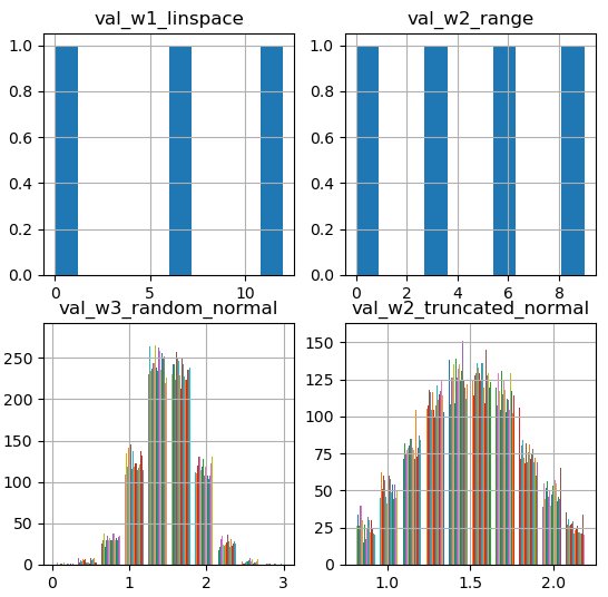
그림. 생성된 ndarray 변수의 분포
변수를 CPU 또는 GPU 디바이스에 할당하거나, 멀티 프로세서인 경우 번호를 지정하여 변수를 할당할 디바이스를 선택한다.
1 2 3 4 5 6 7 8# Device placement # 변수를 특정 디바이스에 할당 with tf.device("/cpu:0"): bias_2= tf.Variable(tf.ones(shape=[200]), name="b2") print(bias_1) # >> Tensor("b1/read:0", shape=(200,), dtype=float32) print(bias_2) # >> Tensor("b2/read:0", shape=(200,), dtype=float32, device=/device:CPU:0)
변수는 tf.train.Saver 클래스를 이용하여 체크포인트 파일로 저장하고 다시 로드할 수 있다.
1 2 3 4 5 6 7 8 9 10 11 12 13 14 15 16 17 18 19 20 21 22 23 24 25 26 27 28""" Saving / Restoring # tf.train.Saver 객체를 이용하여 변수를 체크포인트 파일로 저장/로드 가능 """ model_path = "/tmp/tx-01.ckpt" # 저장 bias_3 = tf.add(bias_1, bias_2, name='b3') init_op = tf.global_variables_initializer() saver = tf.train.Saver() with tf.Session() as sess: sess.run(init_op) val_b3 = sess.run(bias_3) print(val_b3) save_path = saver.save(sess, model_path) print("Model saved in file: %s" % save_path) # 로드 saver = tf.train.Saver() with tf.Session() as sess: saver.restore(sess, model_path) print("Model restored") # access tensor by name directly val_b3 = sess.run('b3:0') print(val_b3) # get tensor by name graph = tf.get_default_graph() b3 = graph.get_tensor_by_name("b3:0") val_b3 = sess.run(b3) print(val_b3)
보는 것과 같이 nativeTF에서는 변수를 생성/초기화 및 특정 디바이스에 할당하는 구문을 작성하는 것이 번거롭다.
TF-Slim에서 변수를 생성, 초기화하는 방법
(예제: c01_defining_models/s01_variables/tf_slim_variables.py)
TF-Slim에서 변수를 생성하고 초기화하는 방법은 좀 더 단순하다. 예를 들어 native-TF에서 변수를 생성하는 아래의 구문은,
1 2with tf.device("/cpu:0"): weight_4 = tf.Variable(tf.truncated_normal(shape=[784, 200], mean=1.5, stddev=0.35), name="w4")
TF-Slim에서는 아래와 같이 생성할 수 있다.
1 2 3 4 5import tensorflow.contrib.slim as slim weight_4 = slim.variable('w4', shape=[784, 200], initializer=tf.truncated_normal_initializer(mean=1.5, stddev=0.35), device='/CPU:0')
모델 변수(model variable)와 일반 변수(regular variable)
변수는 훈련하려는 대상이 되는 파라미터 변수와 훈련 과정에 필요한 변수로 구분할 수 있다. 예를 들어 slim.conv2d, slim.fully_connected 등의 레이어 함수로 생성되는 변수는 훈련하려는 파라미터를 위한 변수를 생성하며, global_step 등과 같은 변수는 훈련 과정에 필요한 변수이며 모델을 구성하는 변수는 아니다. TF-Slim에서는 전자의 경우를 slim.model_variable 함수를 이용하여 모델 변수로 정의할 수 있다.
1 2 3 4 5 6 7 8 9 10 11 12 13 14 15 16 17 18 19# 모델 변수 생성하기 weight_5 = slim.model_variable('w5', shape=[10, 10, 3, 3], initializer=tf.truncated_normal_initializer(stddev=0.1), regularizer=slim.l2_regularizer(0.05), device='/CPU:0') model_variables = slim.get_model_variables() print([var.name for var in model_variables]) # >> [u'w5:0'] # 일반 변수 생성하기 my_var_1 = slim.variable('mv1', shape=[20, 1], initializer=tf.zeros_initializer()) model_variables = slim.get_model_variables() all_variables = slim.get_variables() print([var.name for var in model_variables]) # >> [u'w5:0'] print([var.name for var in all_variables]) # >> [u'w4:0', u'w5:0', u'mv1:0']
레이어
(예제: c01_defining_models/s02_layers/layers.py)
텐서플로우에서 네트워크를 구성할 때 변수와 오퍼레이션 관점에서 레이어를 구성하며, 그 방법은 다음과 같다.
- 가중치와 바이어스에 대한 변수를 생성한다.
- 이전 레이어의 출력을 입력으로 사용하여, 가중치에 대해 컨볼루션 오퍼레이션을 정의한다.
- 위의 출력에 바이어스를 더한다
- 활성화 함수를 적용한다.
1 2 3 4 5 6with tf.variable_scope('conv1_1') as scope: kernel = tf.Variable(tf.truncated_normal([3, 3, 64, 128], dtype=tf.float32, stddev=1e-1, name='weight')) conv = tf.nn.conv2d(input=input_val, filter=kernel, strides=[1, 1, 1, 1], padding='SAME') biases = tf.Variable(tf.constant(0.0, shape=[128], dtype=tf.float32), name='biases') bias = tf.nn.bias_add(conv, biases) conv1 = tf.nn.relu(bias, name='activation')
반면 TF-Slim에서는 레이어 개념을 추상화했으며, 아래와 같이 레이어 관점에서 레이어를 구성할 수 있다.
1 2 3# padding='SAME' is default # strindes=[1,1,1,1] is default net = slim.conv2d(inputs=input_val, num_outputs=128, kernel_size=[3,3], scope='conv1_1')
메타 오퍼레이션: repeat과 stack
TF-Slim은 네트워크 구성을 단순화하기 위한 repeat과 stack 두가지 메타 오퍼레이션을 제공한다. 예를 들어 아래와 네트워크 구성을 보자.
1 2 3 4 5 6 7# VGG network 일부 net1 = tf.placeholder(tf.float32, [16, 32, 32, 256]) with tf.variable_scope('test1') as scope: net1 = slim.conv2d(net1, 256, [3,3], scope='conv3_1') net1 = slim.conv2d(net1, 256, [3,3], scope='conv3_2') net1 = slim.conv2d(net1, 256, [3,3], scope='conv3_3') net1 = slim.max_pool2d(net1, [2,2], scope='pool2')
동일한 인자를 가지는 conv2d 레이어가 중복되고 있다. 이와 같은 경우 아래와 같이 for 루프를 사용하여 해결할 수 있지만,
1 2 3 4 5 6# for loop 사용 net2 = tf.placeholder(tf.float32, [16, 32, 32, 256]) with tf.variable_scope('test2') as scope: for i in range(3): net2 = slim.conv2d(net2, 256, [3,3], scope='conv3_%d' % (i+1)) net2 = slim.max_pool2d(net2, [2,2], scope='pool2')
TF-Slim의 repeat 오퍼레이션을 사용하면 더 단순해진다.
1 2 3 4 5# TF-Slim repeat 사용 net3 = tf.placeholder(tf.float32, [16, 32, 32, 256]) with tf.variable_scope('test3') as scope: net3 = slim.repeat(net3, 3, slim.conv2d, 256, [3,3], scope='conv3') net3 = slim.max_pool2d(net2, [2,2], scope='pool2')
TF-Slim의 stack 오퍼레이션은 더 강력한데, 인자가 다르더라도 동일한 오퍼레이션을 반복할 수 있다. 예를 들어 아래와 같은 MLP 네트워크 구성은
1 2 3 4 5 6 7# MLP 일부 g = tf.Graph() with g.as_default(): input_val = tf.placeholder(tf.float32, [16, 4]) mlp1 = slim.fully_connected(inputs=input_val, num_outputs=32, scope='fc/fc_1') mlp1 = slim.fully_connected(inputs=mlp1, num_outputs=64, scope='fc/fc_2') mlp1 = slim.fully_connected(inputs=mlp1, num_outputs=128, scope='fc/fc_3')
출력 노드가 각각 32, 64, 128로 서로 다르지만 stack 오퍼레이션을 이용하여 아래와 같이 단순화할 수 있다.
1 2 3 4 5# TF-Slim stack 사용 g = tf.Graph() with g.as_default(): input_val = tf.placeholder(tf.float32, [16, 4]) mlp2 = slim.stack(input_val, slim.fully_connected, [32, 64, 128], scope='fc')
컨볼루션 레이어도 유사한 방식으로 stack 오퍼레이션을 적용할 수 있다. 아래의 컨볼루션 네트워크는
1 2 3 4 5 6 7 8# ConvNet 일부 g = tf.Graph() with g.as_default(): input_val = tf.placeholder(tf.float32, [16, 32, 32, 8]) conv1 = slim.conv2d(input_val, 32, [3,3], scope='core/core_1') conv1 = slim.conv2d(conv1, 32, [1, 1], scope='core/core_2') conv1 = slim.conv2d(conv1, 64, [3, 3], scope='core/core_3') conv1 = slim.conv2d(conv1, 64, [1, 1], scope='core/core_4')
아래와 같이 stack을 적용할 수 있다.
1 2 3 4 5# TF-Slim stack 사용 g = tf.Graph() with g.as_default(): input_val = tf.placeholder(tf.float32, [16, 32, 32, 8]) conv2 = slim.stack(input_val, slim.conv2d, [(32,[3,3]), (32,[1,1]), (64,[3,3]), (64,[1,1])], scope='core')
개인적으로는 repeat/stack 오퍼레이션은 프로그래밍 코드보다는 암호처럼 보이는 수준이어서 가독성이 좀 떨어진다는 느낌이다.
스코프(scope)
native TF에서 스코프를 사용하는 방법
(예제: c01_defining_models/s03_scopes/native_tf_scopes.py)
이 절의 내용은 Difference between variable_scope and name_scope in TensorFlow을 참조해서 작성했다. 텐서플로우는 2가지 스코프를 제공하며, 2가지 스코프 모두 변수 앞에 prefix를 붙이는 네이밍 공간 역할을 담당하나 약간의 차이가 있다.
- tf.name_scope
- tf.variable_scope
두 스코프의 가장 큰 차이는 다음과 같다.
- tf.variable_scope는 스코프 내에 있는 모든 변수에 대해 prefix를 추가한다
- tf.Variable(), tf.get_variable() 2가지 방식으로 생성된 변수는 모두 적용된다.
- tf.name_scope는 tf.Variable()로 생성한 변수에 대해서만 prefix를 추가한다
- tf.get_variable()로 생성한 변수는 스코프에 포함되지 않는다(즉, prefix가 추가되지 않는다)
두 스코프의 차이를 비교하는 아래의 코드를 보자.
1 2 3 4 5 6 7 8 9 10 11 12 13 14""" name_scope()와 variable_scope()의 차이 비교 """ def scoping(fn, scope1, scope2, vals): with fn(scope1): a = tf.Variable(vals[0], name='a') b = tf.get_variable('b', initializer=vals[1]) c = tf.constant(vals[2], name='c') with fn(scope2): d = tf.add(a * b, c, name='res') print '\n '.join([scope1, a.name, b.name, c.name, d.name]), '\n' return d d1 = scoping(tf.variable_scope, 'scope_vars', 'res', [1, 2, 3]) d2 = scoping(tf.name_scope, 'scope_name', 'res', [1, 2, 3])
scoping() 유틸 함수를 이용하여, tf.variable_scope를 이용한 네트워크 d1과 tf.name_scope를 이용한 네트워크 d2를 생성한다. 변수 중 a와 c는 tf.Variable을 이용하여 생성했으며, b는 tf.get_variable을 이용하여 생성한다. 출력 결과는 다음과 같다.
1 2 3 4 5 6 7 8 9 10scope_vars scope_vars/a:0 scope_vars/b:0 scope_vars/c:0 scope_vars/res/res:0 scope_name scope_name/a:0 b:0 scope_name/c:0 scope_name/res/res:0
tf.variable_scope의 경우 모든 변수가 스코프 내에 포함되었으나, tf.name_scope의 경우 tf.get_variable을 이용하여 생성한 b는 스코프에 포함되지 않았다. 텐서보드를 이용하여 실제로 그래프를 확인해보자.
1 2 3 4 5 6 7 8 9with tf.Session() as sess: writer = tf.summary.FileWriter('/tmp/tf-slim-tutorial', sess.graph) sess.run(tf.global_variables_initializer()) print sess.run([d1, d2]) writer.close() # 텐서보드 실행 # $ tensorboard --logdir=/tmp/tf-slim-tutorial # 텐서보드 접속 # http://localhost:6006
아르 그래프에서 보는 것처럼 우측의 tf.name_scope의 경우 tf.get_variable을 이용하여 생성한 b는 스코프에 포함되지 않는다.
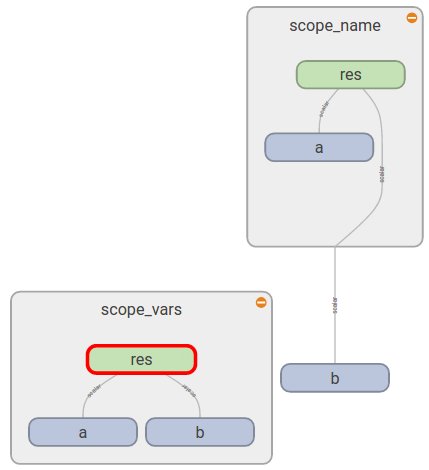
그림. tf.variable_scope와 tf.name_scope의 차이 비교
tf.get_variable 살펴보기
tf.variable_scope와 tf.name_scope의 차이를 좀더 살펴보기 위해 차이가 나는 tf.get_variable를 좀더 살펴보자. tf.get_variable은 이미 정의된 변수를 가져오거나, 없으면 새로 생성한다. 위의 예제에서는 변수 'b'가 생성되어 있지 않으므로 새로 생성한다. 만약 변수 'b'가 생성되어 있는 경우, tf.variable_scope와 tf.name_scope의 차이를 살펴본다. 변수 'b'를 생성한 후 위와 동일한 코드를 실행하면,
1 2 3b = tf.Variable(initial_value=1, name='b') d1 = scoping(tf.variable_scope, 'scope_vars2', 'res', [1, 2, 3]) d2 = scoping(tf.name_scope, 'scope_name2', 'res', [1, 2, 3])
tf.variable_scope의 경우 아래와 같이 출력된다.
1 2 3 4 5scope_vars2 scope_vars2/a:0 scope_vars2/b:0 scope_vars2/c:0 scope_vars2/res/res:0
반면 tf.name_scope의 경우 아래와 같이 에러가 발생한다.
1ValueError: Variable b already exists, disallowed
TF-Slim: slim.arg_scope
(예제: c01_defining_models/s03_scopes/tf_slim_scopes.py)
TF-Slim은 코드 중복을 최대한 방지하기 위해 arg_scope를 추가했다. 네이밍 스페이스를 관리하기 위한 tf.variable_scope와 tf.name_scope보다는 slim.arg_scope는 repeat/stack 메타 오퍼레이션에 더 가까운데, 함수 인자 수준에서 재사용을 최대하 하기위한 구문이다. 아래의 네트워크 구성을 보자.
1 2 3 4 5 6 7 8 9 10 11 12 13 14 15 16import tensorflow as tf import tensorflow.contrib.slim as slim """ 아래의 코드는 하이퍼파라미터/초기화 등 중복이 있이며, 가독성도 떨어짐 """ with tf.variable_scope('test1'): input_val = tf.placeholder(tf.float32, [16, 300, 300, 64]) net1 = slim.conv2d(inputs=input_val, num_outputs=64, kernel_size=[11, 11], stride=4, padding='SAME', weights_initializer=tf.truncated_normal_initializer(stddev=0.01), weights_regularizer=slim.l2_regularizer(0.0005), scope='conv1') net1 = slim.conv2d(inputs=net1, num_outputs=128, kernel_size=[11, 11], padding='VALID', weights_initializer=tf.truncated_normal_initializer(stddev=0.01), weights_regularizer=slim.l2_regularizer(0.0005), scope='conv2') net1 = slim.conv2d(inputs=net1, num_outputs=256, kernel_size=[11, 11], padding='SAME', weights_initializer=tf.truncated_normal_initializer(stddev=0.01), weights_regularizer=slim.l2_regularizer(0.0005), scope='conv3')
3개의 컨볼루션 레이어가 있지만, stride/padding/initalizer/regularizer 등 인자가 다르므로 repeat/stack 오퍼레이션을 사용할 수 없다. 이 경우 인자를 공통 변수로 도출하는 방식으로 리팩토링해볼 수 있다.
1 2 3 4 5 6 7 8 9 10 11 12 13 14 15 16 17 18 19 20 21 22 23""" 1차 리팩토링 # 공통 인자를 변수로 도출 """ with tf.variable_scope('test2'): padding = 'SAME' initializer = tf.truncated_normal_initializer(stddev=0.01) regularizer = slim.l2_regularizer(0.0005) net2 = slim.conv2d(inputs=input_val, num_outputs=64, kernel_size=[11, 11], stride=4, padding=padding, weights_initializer=initializer, weights_regularizer=regularizer, scope='conv1') net2 = slim.conv2d(inputs=net2, num_outputs=128, kernel_size=[11, 11], padding='VALID', weights_initializer=initializer, weights_regularizer=regularizer, scope='conv2') net2 = slim.conv2d(inputs=net2, num_outputs=256, kernel_size=[11, 11], padding=padding, weights_initializer=initializer, weights_regularizer=regularizer, scope='conv3')
첫 번째 코드보다는 중복이 제거되었고 가독성은 높아졌다. slim.arg_scope를 이용하면 이 코드를 더 단순화할 수 있다.
1 2 3 4 5 6 7 8 9 10 11 12""" 2차 리팩토링: slim.arg_scope() 사용 # 공통된 인자는 arg_scope()에 정의. # 다른 인자만 재정의 """ with tf.variable_scope('test3'): with slim.arg_scope([slim.conv2d], padding='SAME', weights_initializer=tf.truncated_normal_initializer(stddev=0.01), weights_regularizer=slim.l2_regularizer(0.0005)): net3 = slim.conv2d(inputs=input_val, num_outputs=64, kernel_size=[11, 11], stride=4, scope='conv1') net3 = slim.conv2d(inputs=net3, num_outputs=128, kernel_size=[11, 11], padding='VALID', scope='conv2') net3 = slim.conv2d(inputs=net3, num_outputs=256, kernel_size=[11, 11], scope='conv3')ㅎ
레이어 함수의 공통 인자는 slim.arg_scope에 지정하고, 다른 인자만 오버라이드(override)하는 방식이다.
또한 slim.arg_scope는 중첩이 가능하므로, 아래와 같이 네트워크를 구성한는 것도 가능해진다.
1 2 3 4 5 6 7 8 9 10 11 12 13 14""" slim.arg_scope() 중첩 가능 """ with tf.variable_scope('test5'): with slim.arg_scope([slim.conv2d, slim.fully_connected], activation_fn=tf.nn.relu, weights_initializer=tf.truncated_normal_initializer(stddev=0.01), weights_regularizer=slim.l2_regularizer(0.0005)): with slim.arg_scope([slim.conv2d], stride=1, padding='SAME'): net4 = slim.conv2d(inputs=input_val, num_outputs=64, kernel_size=[11, 11], stride=4, scope='conv1') net4 = slim.conv2d(inputs=net4, num_outputs=256, kernel_size=[5, 5], weights_initializer=tf.truncated_normal_initializer(stddev=0.03), scope='conv2') net4 = slim.fully_connected(inputs=net4, num_outputs=1000, activation_fn=None, scope='fc')
네트워크 구성 예제
MNIST 필기체 인식
가장 간단한 예로 MNIST 필기체 인식 문제를 살펴보자. 구성하려는 네트워크는 다음과 같다. 2개의 컨볼루션 레이어와 2개의 fully-connected 레이어, 그리고 드롭아웃(Dropout)이 적용되었다.
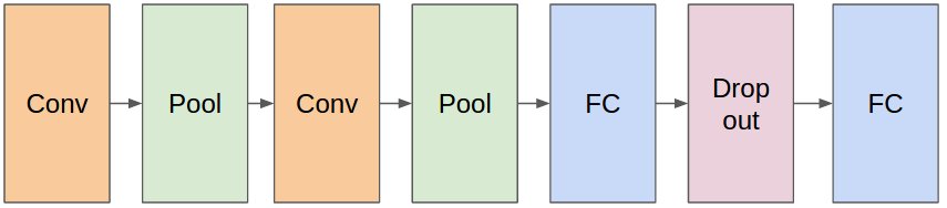
그림. MNIST ConvNet 구조
먼저 native-TF로 구현한 예제는 다음과 같으며, 자세한 내용은 텐서플로우(TensorFlow) 시작하기에서 확인할 수 있다.
(예제: c01_defining_models/s04_examples/mnist_deep_step_by_step.py)
1 2 3 4 5 6 7 8 9 10 11 12 13 14 15 16 17 18 19 20 21 22 23 24 25 26 27 28 29 30 31 32 33 34 35 36 37 38 39 40 41 42 43# Define weight(kernel filter) with shape def weight_variable(shape): initial = tf.truncated_normal(shape, stddev=0.1) return tf.Variable(initial) # Define bias with shape def bias_variable(shape): initial = tf.constant(0.1, shape=shape) return tf.Variable(initial) # Define convolution with x and W def conv2d(x, W): return tf.nn.conv2d(x, W, strides=[1, 1, 1, 1], padding='SAME') # Define max pooling with x and W def max_pool_2x2(x): return tf.nn.max_pool(x, ksize=[1, 2, 2, 1], strides=[1, 2, 2, 1], padding='SAME') # 1st ConvNet layer ## 32 Kernel Filter with size 5x5 on 1 input channel W_conv1 = weight_variable([5, 5, 1, 32]) b_conv1 = bias_variable([32]) h_conv1 = tf.nn.relu(conv2d(x_image, W_conv1) + b_conv1) # 1st Pooling layer ## 2x2 max pooling h_pool1 = max_pool_2x2(h_conv1) # 2nd ConvNet layer ## 64 Kernel Filter with size 5x5 on 32 input channel W_conv2 = weight_variable([5, 5, 32, 64]) b_conv2 = bias_variable([64]) h_conv2 = tf.nn.relu(conv2d(h_pool1, W_conv2) + b_conv2) # 2nd Pooling layer ## 2x2 max pooling h_pool2 = max_pool_2x2(h_conv2) # Densely connected layer W_fc1 = weight_variable([7 * 7 * 64, 1024]) b_fc1 = bias_variable([1024]) h_pool2_flat = tf.reshape(h_pool2, [-1, 7*7*64]) h_fc1 = tf.nn.relu(tf.matmul(h_pool2_flat, W_fc1) + b_fc1) ## Apply dropout keep_prob = tf.placeholder(tf.float32) h_fc1_drop = tf.nn.dropout(h_fc1, keep_prob) # Output layer W_fc2 = weight_variable([1024, 10]) b_fc2 = bias_variable([10]) y_conv = tf.matmul(h_fc1_drop, W_fc2) + b_fc2
보는 것과 같이 레이어 관점이 아닌 변수와 오퍼레이션 관점에서 네트워크를 구성해야 한다. 동일한 네트워크를 TF-Slim을 이용하면, 레이어 관점에서 구성할 수 있으며, 다음과 같이 간단해진다.
(예제: c01_defining_models/s04_examples/mnist_deep_step_by_step_slim.py)
1 2 3 4 5 6 7 8 9 10 11 12 13 14 15def mnist_convnet(inputs, is_training=True): with slim.arg_scope([slim.conv2d, slim.fully_connected], activation_fn=tf.nn.relu, weights_initializer=tf.truncated_normal_initializer(stddev=0.1)): with slim.arg_scope([slim.conv2d], kernel_size=5): net = slim.conv2d(inputs=inputs, num_outputs=32, scope='conv1') net = slim.max_pool2d(inputs=net, kernel_size=[2,2], scope='pool1') net = slim.conv2d(inputs=net, num_outputs=64, scope='conv2') net = slim.max_pool2d(inputs=net, kernel_size=[2, 2], scope='pool2') net = slim.flatten(inputs=net, scope='flatten') net = slim.fully_connected(inputs=net, num_outputs=1024, scope='fc3') net = slim.dropout(inputs=net, is_training=is_training, keep_prob=0.5, scope='dropout4') net = slim.fully_connected(inputs=net, num_outputs=10, activation_fn=None, scope='fc4') return net
VGG 네트워크
이미지 분류 태스크의 경우 네트워크를 직접 구상하기보다는 성능이 검증된 주요 네트워크 아키텍처를 그대로 가져다 쓰는 편이 좋다. TF-Slim 라이브러리는 자주 사용하는 이미지 모델(VGG, Incetion, ResNet 등)을 쉽게 활용할 수 있도록 slim.nets 모듈을 제공한다. 예를 들어 기본 네트워크 모델로 VGG-16 모델을 사용하는 경우 아래와 같이 모델을 임포트할 수 있다.
1 2 3 4 5import tensorflow.contrib.slim.nets vgg = tf.contrib.slim.nets.vgg images, labels = load_batch(..) with slim.arg_scope(vgg.vgg_arg_scope()): logits, end_points = vgg.vgg_16(inputs=images, num_classes=num_classes, is_training=True)
주의할 점은 slim.nets에 정의된 네트워크는 tf-slim 모듈을 이용하여 리팩토링되었으며, 코드 중복을 피하기 위해 slim.arg_scope 기능을 사용하고 있다. 따라서 임포트하려는 네트워크 아키텍처에 맞는 slim.arg_scope 내부에서 모델을 임포트해야 한다.
VGG-16 네트워크 모델을 포함한 기본 모델은 이미지넷 데이터셋을 기반으로 하므로 출력 레이블의 개수인 num_classes는 1000이다. 반면 이러한 네트워크를 기반 모델로 사용하여 자신의 태스크에 사용하는 경우 레이블의 개수는 문제에 따라 달라진다.
또한 자신의 훈련 데이터셋을 이용하여 처음부터 학습하기 보다는, 이미지넷 데이터셋을 기반으로 학습된 체크포인트 파일을 가중치로 초기화한 후 fine-tuning하면 훈련이 더 빠르게 수렴한다. 학습된 모델을 이용하여 fine-tuning하는 방법은 개 품종 분류 예제를 다루면서 자세히 설명한다.
훈련 데이터 로드하기
이 절에서는 학습 데이터셋을 TFRecord 포맷으로 변환하고, 훈련 과정에서 데이터를 피드하는 방법을 설명한다. 이 절의 내용은 TensorFlow-Slim image classification library을 참고했다.
TFRecord 포맷
학습할 데이터셋을 훈련할 수 있는 포맷으로 변환해야 한다. 다양한 포맷과 변환 방법이 있지만 대체적으로 아래의 구조를 따른다.
- 전체 데이터셋을 훈련/평가 데이터셋으로 분할
- 데이터를 네트워크 입력 레이어의 사이즈에 맞게 전처리
- 미니배치 훈련을 위한 배치 사이즈 크기의 데이터 피드 기능 제공
- 결과 레이블에 대한 one-hot encoding 변환
이 중 전처리와 one-hot encoding 변환은 훈련 과정에서 동적으로 처리할 수도 있다. 이 글에서는 학습 데이터셋을 텐서플로우 표준 데이터 포맷인 TFRecord 포맷으로 변환하여 사용하는 방법을 소개한다.
MNIST 학습 데이터셋 구하기
먼저 학습 데이터셋을 구한다. 이미지 분류 문제의 경우 학습 데이터셋은 이미지 파일이다. 이 절에서는 MNIST 이미지 데이터셋을 학습 데이터셋으로 사용한다. Kaggle > MNIST as .jpg에서 jpg 포맷의 데이터를 제공한다. 이 중에서 42,000개로 구성된 훈련 데이터셋 trainingSet.tar.gz.zip을 다운로드한 후 압축을 푼다. 이 데이터를 수집 가능한 데이터셋 전체라고 가정한 후, 훈련용 데이터셋과 평가용 데이터셋으로 분할하여 사용한다.
TFRecord 포맷으로 변환하기
수집한 입력 이미지 데이터셋을 TFRecord 포맷으로 변환한다. 이때 훈련 데이터셋은 아래와 같이 구조화되어야 한다.
(예제: c02_loading_datasets/s01_tfrecord/create_tf_record.py)
1 2 3 4 5 6 7 8 9 10 11 12 13 14 15 16 17 18# 훈련 데이터셋의 구조 raw_data/ |- flowers/ |- images/ |- class-1/ |- class-2/ |- class-3/ |- class-4/ |-- ... # MNITS의 경우 raw_data/ |- mnist/ |- images/ |- 0/ |- 1/ |- 2/ |- 3/ |-- ...
즉 각 레이블별로 디렉토리가 있으며, 각 디렉토리에 해당 레이블에 해당하는 이미지가 위치한다. 디렉토리명은 레이블 명에 해당한다. 변환 프로그램은 4개의 인자를 받는다.
- dataset_name 생성된 TFRecord 파일명의 prefix 예) --dataset_name=mnist
- dataset_dir 위의 tree 형태의 raw 데이터셋이 저장된 디렉토리 위치 (이때 각 레이블 디렉토리는 images/ 디렉토리 하위에 위치한다고 가정) 예) --dataset_dir=./raw_data/mnist
- num_shards 생성할 TFRecord 샤드 개수 예) --num_shards=5
- ratio_val 평가 데이터셋의 비율 예) --ratio_val=0.2
1 2 3 4 5 6 7 8 9 10 11 12 13 14 15 16 17 18 19 20 21 22 23 24 25 26from datasets import convert_tf_record FLAGS = tf.app.flags.FLAGS tf.app.flags.DEFINE_string( 'dataset_name', 'mnist', 'The name of the dataset prefix.') tf.app.flags.DEFINE_string( 'dataset_dir', './raw_data/mnist', 'A directory containing a set of subdirectories representing class names. Each subdirectory should contain PNG or JPG encoded images.') tf.app.flags.DEFINE_integer( 'num_shards', 5, 'A number of sharding for TFRecord files(integer).') tf.app.flags.DEFINE_float( 'ratio_val', 0.2, 'A ratio of validation datasets for TFRecord files(flaot, 0 ~ 1).') def main(_): if not FLAGS.dataset_name: raise ValueError('You must supply the dataset name with --dataset_name') if not FLAGS.dataset_dir: raise ValueError('You must supply the dataset directory with --dataset_dir') convert_tf_record.run(FLAGS.dataset_name, FLAGS.dataset_dir, FLAGS.num_shards, FLAGS.ratio_val) if __name__ == '__main__': tf.app.run()
실제로 변환을 수행하는 코드는 datasets/convert_tf_record.py의 run() 함수에서 수행한다.
(예제: c02_loading_datasets/s01_tfrecord/convert_tf_record.py)
해당 코드는 flowers 데이터셋을 다운로드한 후 TFRecord 포맷으로 변환하는 https://github.com/tensorflow/models/blob/master/slim/datasets/download_and_convert_flowers.py을 약간 수정했다. 주요 변경 사항은 학습 데이터셋 전체에 대해 ratio_val을 입력 받아서, 훈련용/평가용 데이터셋을 분할 생성하도록 했다.
1 2 3 4 5 6 7 8 9 10 11 12# Cacluate number of validation proportional to ratio_val num_validation = int(len(photo_filenames) * ratio_val) # Divide into train and test: random.seed(_RANDOM_SEED) random.shuffle(photo_filenames) training_filenames = photo_filenames[num_validation:] validation_filenames = photo_filenames[:num_validation] # First, convert the training and validation sets. _convert_dataset('train', training_filenames, class_names_to_ids, dataset_dir, dataset_name, tf_record_dir, num_shards) _convert_dataset('validation', validation_filenames, class_names_to_ids, dataset_dir, dataset_name, tf_record_dir, num_shards)
아래와 같이 변환 작업을 실행하면 8:2의 비율로 TFRecord 파일이 $DATASET_DIR/tfrecord/ 디렉토리에 생성된다.
1 2 3 4 5 6 7 8 9 10 11 12 13 14 15 16 17 18 19 20 21 22$ DATASET_DIR=/home/itrocks/Git/Tensorflow/tf-slim-tutorial/raw_data/mnist $ python c02_loading_datasets/s01_tfrecord/create_tf_record.py --dataset_name=mnist \ --dataset_dir=$DATASET_DIR \ --num_shards=5 \ --ratio_val=0.2 ... >> Converting [train] image 33600/33600 shard 4 .. >> Converting [validation] image 8400/8400 shard 4 $ $ tree $DATASET_DIR/tfrecord/ /home/itrocks/Git/Tensorflow/tf-slim-tutorial/raw_data/mnist/tfrecord/ ├── labels.txt ├── mnist_train_00000-of-00005.tfrecord ├── mnist_train_00001-of-00005.tfrecord ├── mnist_train_00002-of-00005.tfrecord ├── mnist_train_00003-of-00005.tfrecord ├── mnist_train_00004-of-00005.tfrecord ├── mnist_validation_00000-of-00005.tfrecord ├── mnist_validation_00001-of-00005.tfrecord ├── mnist_validation_00002-of-00005.tfrecord ├── mnist_validation_00003-of-00005.tfrecord └── mnist_validation_00004-of-00005.tfrecord
이미지를 TFRecord 포맷으로 변환하는 작업은 예제 c02_loading_datasets/s01_tfrecord/convert_tf_record.py의 _convert_dataset(...) 메서드에서 실행한다.
1 2 3 4 5 6 7 8 9with tf.python_io.TFRecordWriter(output_filename) as tfrecord_writer: ... image_data = tf.gfile.FastGFile(filenames[i], 'rb').read() height, width = image_reader.read_image_dims(sess, image_data) class_id = class_names_to_ids[class_name] example = dataset_utils.image_to_tfexample( image_data, b'jpg', height, width, class_id) tfrecord_writer.write(example.SerializeToString()) ...
이미지 파일들에 대해 루프를 돌면서
- image_data 바이너리 이미지 데이터
- height / weight 이미지의 가로/세로
- class_id 실제 레이블 ID
등의 정보를 포함하는 tf.train.Example객체를 dataset_utils.image_to_tfexample() 메서드를 통해 생성한다. (예제: datasets/dataset_utils.py)
1 2 3 4 5 6 7 8def image_to_tfexample(image_data, image_format, height, width, class_id): return tf.train.Example(features=tf.train.Features(feature={ 'image/encoded': bytes_feature(image_data), 'image/format': bytes_feature(image_format), 'image/class/label': int64_feature(class_id), 'image/height': int64_feature(height), 'image/width': int64_feature(width), }))
DatasetDataProvider
입력 데이터셋을 TFRecord 포맷으로 변환했다면, 아래와 과정을 따라 TFRecord 데이터를 읽어서 데이터를 피드한다.
- TFRecord 포맷 데이터을 읽어서 변환할 수 있도록 slim.dataset.Dataset 클래스를 정의한다.
- 데이터를 피드하기 위한 slim.dataset_data_provider.DatasetDataProvider를 생성한다.
- 네트워크 모델의 입력에 맞게 전처리 작업 및 편의를 위한 one-hot 인코딩 작업을 한 후, tf.train.batch를 생성한다.
slim.dataset.Dataset 클래스를 정의
먼저 slim.dataset.Dataset 객체를 생성한다. (예제: c02_loading_datasets/s02_dataset_provider/load_tf_record_dataset.py)
1 2 3 4 5 6 7 8 9""" # slim.dataset.Dataset 클래스를 정의 """ TF_RECORD_DIR = '/home/itrocks/Git/Tensorflow/tf-slim-tutorial/raw_data/mnist/tfrecord' mnist_tfrecord_dataset = tf_record_dataset.TFRecordDataset(tfrecord_dir=TF_RECORD_DIR, dataset_name='mnist', num_classes=10) # train 데이터셋 생성 dataset = mnist_tfrecord_dataset.get_split(split_name='train')
tf_record_dataset.get_split(...) 메서드에서 slim.dataset.Dataset 객체를 생성한다. (예제: dataset/tf_record_dataset.py)
1 2 3 4 5 6 7 8 9 10 11 12 13 14 15 16 17 18 19 20 21 22 23 24 25 26 27 28 29 30def get_split(self, split_name): splits_to_sizes = self.__get_num_samples__(split_name) if split_name not in ['train', 'validation']: raise ValueError('split name %s was not recognized.' % split_name) file_pattern = self.dataset_name + '_' + split_name + '_*.tfrecord' file_pattern = os.path.join(self.tfrecord_dir, file_pattern) reader = tf.TFRecordReader keys_to_features = { 'image/encoded': tf.FixedLenFeature((), tf.string, default_value=''), 'image/format': tf.FixedLenFeature((), tf.string, default_value='jpg'), 'image/class/label': tf.FixedLenFeature( [], tf.int64, default_value=tf.zeros([], dtype=tf.int64)), } items_to_handlers = { 'image': slim.tfexample_decoder.Image(), 'label': slim.tfexample_decoder.Tensor('image/class/label'), } decoder = slim.tfexample_decoder.TFExampleDecoder( keys_to_features, items_to_handlers) labels_to_names = None if dataset_utils.has_labels(self.tfrecord_dir): labels_to_names = dataset_utils.read_label_file(self.tfrecord_dir) return slim.dataset.Dataset( data_sources=file_pattern, reader=reader, decoder=decoder, num_samples=splits_to_sizes, items_to_descriptions=_ITEMS_TO_DESCRIPTIONS, num_classes=self.num_classes, labels_to_names=labels_to_names)
- reader tf.TFRecordReader를 이용해 TFRecord 파일을 읽는다
- decoder TFRecord 포맷으로 인코딩된 tf.train.Example 객체를 slim.tfexample_decoder.TFExampleDecoder 객체를 이용하여 디코딩한다. TFExampleDecoder는 keys_to_feature와 items_to_handlers를 인자로 받으며, 이를 이용하여 tf.train.Example 객체를 [key:tensor] 형태로 디코딩한다.
slim.dataset_data_provider.DatasetDataProvider를 생성
실제로 데이터를 디코딩하고 데이터를 피드하는 역할은 slim.dataset_data_provider.DatasetDataProvider가 수행한다. (예제: c02_loading_datasets/s02_dataset_provider/load_tf_record_dataset.py)
1 2 3 4 5""" # slim.dataset_data_provider.DatasetDataProvider를 생성 """ provider = slim.dataset_data_provider.DatasetDataProvider(dataset) [image, label] = provider.get(['image', 'label'])
items_to_handlers 사전에 정의된 key값으로 텐서를 리턴한다.
pyplot을 이용해서 디코딩된 텐서를 실제로 표시해 본다. (예제: c02_loading_datasets/s02_dataset_provider/load_tf_record_dataset.py)
1 2 3 4 5 6 7 8 9 10 11 12 13 14# 테스트 import matplotlib.pyplot as plt with tf.Session() as sess: with slim.queues.QueueRunners(sess): plt.figure() for i in range(4): np_image, np_label = sess.run([image, label]) height, width, _ = np_image.shape class_name = name = dataset.labels_to_names[np_label] plt.subplot(2, 2, i+1) plt.imshow(np_image) plt.title('%s, %d x %d' % (name, height, width)) plt.axis('off') plt.show()
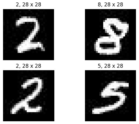
그림. 첫 4개의 이미지 출력
전처리/인코딩 및 tf.train.batch 생성
미니 배치 학습을 위해 배치 사이즈만큼의 tf.train.batch 객체를 생성한다. (예제: c02_loading_datasets/s02_dataset_provider/load_tf_record_dataset.py)
1 2 3 4''' tf.train.batch를 생성 ''' images, labels, _ = load_batch(dataset)
load_batch 메서드는 예제: utils/dataset_utils.py에 정의되어 있다. tf.train.batch를 생성할 때, 데이터를 모델의 입력 사이즈(가로, 세로, 채널)에 맞게 변환한다. 그리고 출력 레이블은 나중에 손실 계산에 용이하도록 one-hot 포맷으로 인코딩으로 변환한다.
1 2 3 4 5 6 7 8 9 10 11 12 13 14 15 16 17 18 19 20 21 22 23 24 25 26 27 28def load_batch(dataset, batch_size=32, height=28, width=28, num_classes=10, is_training=True): """Loads a single batch of data. Args: dataset: The dataset to load. batch_size: The number of images in the batch. height: The size of each image after preprocessing. width: The size of each image after preprocessing. is_training: Whether or not we're currently training or evaluating. Returns: images: A Tensor of size [batch_size, height, width, 3], image samples that have been preprocessed. images_raw: A Tensor of size [batch_size, height, width, 3], image samples that can be used for visualization. labels: A Tensor of size [batch_size], whose values range between 0 and dataset.num_classes. """ # Creates a TF-Slim DataProvider which reads the dataset in the background during both training and testing. provider = slim.dataset_data_provider.DatasetDataProvider(dataset) [image, label] = provider.get(['image', 'label']) # image: resize with crop image = tf.image.resize_image_with_crop_or_pad(image, height, width) image = tf.to_float(image) # label: one-hot encoding one_hot_labels = slim.one_hot_encoding(label, num_classes) # Batch it up. images, labels = tf.train.batch( [image, one_hot_labels], batch_size=batch_size, num_threads=1, capacity=2 * batch_size) return images, labels, dataset.num_samples
훈련 이미지 전처리 과정은 학습 성능을 높이는데 중요한 역할을 하며, 준비된 이미지를 다양한 방식으로 변환(crop, flip, color distortion)하면 학습 성능을 높이는데 도움이 된다. 데이터 augmentation 관련해서는 models/research/slim/preprocessing/inception_preprocessing.py 코드가 도움이 된다. 예를 들어 color distortion의 경우, distort_color(...) 메서드를 이용할 수 있으며, 훈련 이미지에 대해 색상(hue), 채도(saturation), 밝기(brightness), 대비(contrast)를 랜덤하게 적용한다.
1 2 3 4image = tf.image.random_hue(image, max_delta=0.2) image = tf.image.random_saturation(image, lower=0.5, upper=1.5) image = tf.image.random_contrast(image, lower=0.5, upper=1.5) image = tf.image.random_brightness(image, max_delta=32. / 255.)
모델 훈련하기
모델을 훈련하려면 모델과 손실 함수를 정의한 후, 훈련 데이터를 이용하여 반복적으로 모델의 파라미터를 업데이트해야 한다. TF-Slim을 이용하여 모델을 정의하는 방법은 앞에서 다뤘고, 이 장에서는 모델을 훈련하는 방법을 설명한다. 훈련할 네트워크를 정의했다면, 이후의 과정은 아래와 같이 기본 학습과정과 동일하다. (예제: c03_training_models/train_mnist.py)
- 손실함수 정의
- 옵티마이저 정의
- 메트릭 정의
- 훈련하기
TF-Slim은 일반적인 손실함수와 훈련/평가 루틴을 간편하게 실행할 수 있는 헬퍼 함수들을 제공한다.
손실함수 정의
slim.losses 패키지의 손실함수를 이용한다.
1 2loss = slim.losses.softmax_cross_entropy(logits, labels) total_loss = slim.losses.get_total_loss()
옵티마이저 정의
옵티마이저는 tf.train 패키지의 옵티마이저를 그대로 사용한다.
1optimizer = tf.train.AdamOptimizer(learning_rate=0.0001)
메트릭 정의
텐서보드 시각화를 위한 메트릭을 정의한다.
1 2 3 4 5 6 7predictions = tf.argmax(logits, 1) targets = tf.argmax(labels, 1) correct_prediction = tf.equal(predictions, targets) accuracy = tf.reduce_mean(tf.cast(correct_prediction, tf.float32)) tf.summary.scalar('losses/Total', total_loss) tf.summary.scalar('accuracy', accuracy) summary_op = tf.summary.merge_all()
훈련하기
훈련은 slim.learing.train(...) 함수를 이용한다.
1 2 3 4 5 6 7 8 9 10 11 12 13 14# logging 경로 설정 log_dir = '/tmp/tfslim_model/' if not tf.gfile.Exists(log_dir): tf.gfile.MakeDirs(log_dir) # 훈련 오퍼레이션 정의 train_op = slim.learning.create_train_op(total_loss, optimizer) final_loss = slim.learning.train( train_op, log_dir, number_of_steps=2000, summary_op=summary_op, save_summaries_secs=30, save_interval_secs=30) print('Finished training. Final batch loss %f' % final_loss)
훈련을 실행한다.
1 2 3 4 5 6 7 8 9$ python c03_training_models/train_mnist.py ... INFO:tensorflow:global step 1997: loss = 4.4045 (0.086 sec/step) INFO:tensorflow:global step 1998: loss = 3.5334 (0.092 sec/step) INFO:tensorflow:global step 1999: loss = 1.2915 (0.101 sec/step) INFO:tensorflow:global step 2000: loss = 3.3887 (0.101 sec/step) INFO:tensorflow:Stopping Training. INFO:tensorflow:Finished training! Saving model to disk. Finished training. Final batch loss 3.388688
훈련이 실행되면 텐서보드를 실행하여 훈련 과정을 모니터링한다.
1$ tensorboard --logdir=/tmp/tfslim_model
http://localhost:6006/로 접속하여 훈련 메트릭을 모니터링할 수 있다.
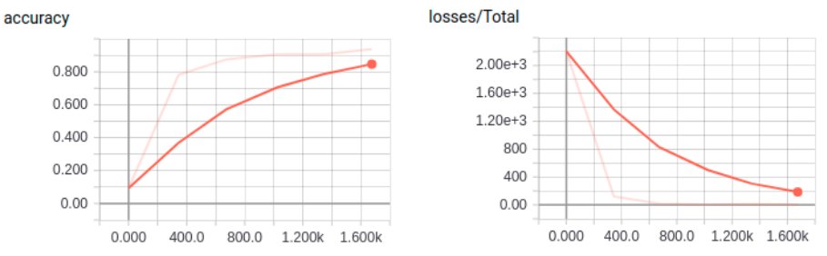
그림. 텐서보드로 MNIST 훈련 모니터링
모델 평가하기
모델 훈련이 완료되면, 평가 데이터셋을 이용하여 모델을 평가한다. (예제: c05_evaluating_models/eval_mnist.py)
훈련과 마찬가지로 모델 평가 과정에서도 metric을 업데이트하고 평가를 간단하게 할 수 있는 유틸리티 함수들을 제공한다. 자세한 내용은 TensorFlow-Slim에서 확인할 수 있다. 아래는 MNIST 데이터에 대해 학습된 체크포인트를 평가하는 코드다.
1 2 3 4 5 6 7 8 9 10 11 12 13 14 15 16 17 18 19 20 21 22 23 24 25 26 27 28 29 30 31 32 33 34 35 36 37 38 39 40 41 42 43 44 45 46''' # 평가 데이터 로드 ''' mnist_tfrecord_dataset = tf_record_dataset.TFRecordDataset( tfrecord_dir='/home/itrocks/Git/Tensorflow/tf-slim-tutorial/raw_data/mnist/tfrecord', dataset_name='mnist', num_classes=10) # Selects the 'train' dataset. dataset = mnist_tfrecord_dataset.get_split(split_name='validation') images, labels, _ = load_batch(dataset) ''' # 모델 정의 ''' predictions = mnist_model.mnist_convnet(inputs=images, is_training=False) ''' # 메트릭 정의 ''' predictions = tf.argmax(predictions, 1) labels = tf.argmax(labels, 1) # Define the metrics: names_to_values, names_to_updates = slim.metrics.aggregate_metric_map({ 'eval/Accuracy': slim.metrics.streaming_accuracy(predictions, labels), # 'eval/Recall@5': slim.metrics.streaming_recall_at_k(predictions, labels, 5), }) ''' # 평가하기 ''' # logging 경로 설정 log_dir = '/tmp/tfslim_model/' eval_dir = '/tmp/tfslim_model-eval/' if not tf.gfile.Exists(eval_dir): tf.gfile.MakeDirs(eval_dir) if not tf.gfile.Exists(log_dir): raise Exception("trained check point does not exist at %s " % log_dir) else: checkpoint_path = tf.train.latest_checkpoint(log_dir) metric_values = slim.evaluation.evaluate_once( master='', checkpoint_path=checkpoint_path, logdir=eval_dir, num_evals=100, eval_op=names_to_updates.values(), final_op=names_to_values.values()) names_to_values = dict(zip(names_to_values.keys(), metric_values)) for name in names_to_values: print('%s: %f' % (name, names_to_values[name]))
모델을 평가한다.
1 2 3 4 5 6 7 8 9 10$ python c05_evaluating_models/eval_mnist.py ... INFO:tensorflow:Restoring parameters from /tmp/tfslim_model/model.ckpt-2000 INFO:tensorflow:Evaluation [1/100] INFO:tensorflow:Evaluation [2/100] ... INFO:tensorflow:Evaluation [99/100] INFO:tensorflow:Evaluation [100/100] INFO:tensorflow:Finished evaluation at 2017-10-18-08:11:12 eval/Accuracy: 0.955938
학습된 모델 Fine-Tuning
지금까지는 임의로 초기화된 파라미터를 scratch로부터 학습했다. 실제 문제에서는 pre-trained된 모델의 체크포인트로부터 파라미터를 초기화한 후, 파라미터를 학습하는 것이 낫다. 이 장부터는 VGG-16 네트워크를 모델을 기반으로 개 이미지 사진을 학습 데이터로 이용하여 개 품종을 분류하는 방법을 소개한다. 개 품종 분류 예제는 dog-breed-classification.tf에서 클론할 수 있다.
학습 데이터 준비하기
학습 이미지 준비하기
개 품종 이미지는 Standford Dogs Dataset에서 다운로드할 수 있다. 학습 데이터에는 이미지와 어노테이션 파일이 있으며, 총 120개의 카테고리와 20,580개의 이미지로 구성된다. 이미지 데이터와 어노테이션은 카테고리별로 디렉토리가 있고, 각 디렉토리에 해당 카테고리의 개 이미지가 들어 있다.
1 2 3 4 5 6 7 8$ tree -L 1 Images/ Images/ ├── n02085620-Chihuahua ├── n02085782-Japanese_spaniel ├── n02085936-Maltese_dog ├── n02086079-Pekinese ├── n02086240-Shih-Tzu ├── ...
1 2 3 4 5 6 7 8$ tree -L 1 Annotation/ Annotation/ ├── n02085620-Chihuahua ├── n02085782-Japanese_spaniel ├── n02085936-Maltese_dog ├── n02086079-Pekinese ├── n02086240-Shih-Tzu ├── ...
이미지 1개당 1개의 어노테이션 파일이 있으며, 어노테이션 파일은 Pascal VOC 포맷의 XML 파일로 작성되어 있다.
1 2 3 4 5 6 7 8 9 10 11 12 13 14 15 16 17 18 19 20 21 22 23 24 25<annotation> <folder>02085620</folder> <filename>n02085620_7</filename> <source> <database>ImageNet database</database> </source> <size> <width>250</width> <height>188</height> <depth>3</depth> </size> <segment>0</segment> <object> <name>Chihuahua</name> <pose>Unspecified</pose> <truncated>0</truncated> <difficult>0</difficult> <bndbox> <xmin>71</xmin> <ymin>1</ymin> <xmax>192</xmax> <ymax>180</ymax> </bndbox> </object> </annotation>
이미지 Crop하기
이미지 파일은 object localization을 위한 영역정보(bndbox)까지 포함하고 있으나, 이 예제에서는 분류(classification)이 목적이므로, 이미지에서 해당 영역만을 잘라서 이미지 데이터를 재구성한다. 예제 프로젝트의 crop.py을 실행한다. 이때 Standford Dogs Dataset에서 다운로드받은 위치를 root_dir에, crop된 이미지를 저장할 디렉토리를 target_image_dir에 설정한 후 crop.py를 실행한다.
1 2root_dir = '/home/itrocks/Backup/Data/StandfordDogs' target_image_dir = '/home/itrocks/Git/Tensorflow/dog-breed-classification.tf/raw_data/dog/images'
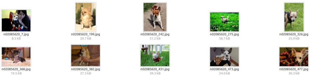
그림. 원본 이미지 예시
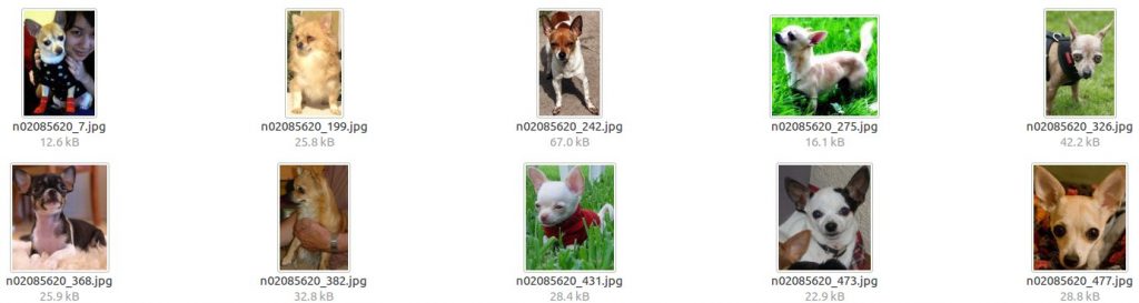
그림. bndbox 영역만 Crop한 이미지 예시
TFRecord 변환하기
crop된 이미지를 TFRecord 데이터로 변환한다. create_tf_record.py를 이용하여 변환할 수 있으며, MNIST에서 작성한 코드 그대로다.
1 2 3 4 5 6 7 8 9 10 11 12 13 14 15 16 17 18 19 20 21 22 23 24$DATASET_DIR=/home/itrocks/Git/Tensorflow/dog-breed-classification.tf/raw_data/dog $python create_tf_record.py --dataset_name=dog \ --dataset_dir=$DATASET_DIR \ --num_shards=5 \ --ratio_val=0.2 ... >> Converting [train] image 16464/16464 shard 4 ... >> Converting [validation] image 4116/4116 shard 4 ... $ tree $DATASET_DIR/tfrecord/ /home/itrocks/Git/Tensorflow/dog-breed-classification.tf/raw_data/dog/tfrecord/ ├── dog_train_00000-of-00005.tfrecord ├── dog_train_00001-of-00005.tfrecord ├── dog_train_00002-of-00005.tfrecord ├── dog_train_00003-of-00005.tfrecord ├── dog_train_00004-of-00005.tfrecord ├── dog_validation_00000-of-00005.tfrecord ├── dog_validation_00001-of-00005.tfrecord ├── dog_validation_00002-of-00005.tfrecord ├── dog_validation_00003-of-00005.tfrecord ├── dog_validation_00004-of-00005.tfrecord └── labels.txt 0 directories, 11 files
훈련 데이터 로드하기
TFRecord로 변환된 데이터를 훈련에 사용할 수 있게 로드한다.
1 2 3 4 5 6 7 8 9 10 11''' # 훈련 데이터 로드 ''' batch_size = 16 tfrecord_dataset = tf_record_dataset.TFRecordDataset( tfrecord_dir='/home/itrocks/Git/Tensorflow/dog-breed-classification.tf/raw_data/dog/tfrecord', dataset_name='dog', num_classes=120) # Selects the 'train' dataset. dataset = tfrecord_dataset.get_split(split_name='train') images, labels, num_samples = load_batch(dataset, batch_size=batch_size, height=224, width=224)
VGG-16 네트워크의 입력이미지는 224 x 224다. 그리고 전처리 과정에 vgg_preprocessing.py에 정의된 메서드를 활용한다. utils/dataset_utils의 load_batch(...) 메서드를 아래와 같이 수정한다.
1 2 3 4 5# image: resize with crop #image = tf.image.resize_image_with_crop_or_pad(image, height, width) #image = tf.to_float(image) import preprocess.vgg_preprocessing as vgg_preprocessing image = vgg_preprocessing.preprocess_for_train(image, height, width)
vgg_preprocessing.preprocess_for_train(...) 메서드는 아래와 같이 구현되어 있다.
1 2 3 4 5 6image = _aspect_preserving_resize(image, resize_side) image = _random_crop([image], output_height, output_width)[0] image.set_shape([output_height, output_width, 3]) image = tf.to_float(image) image = tf.image.random_flip_left_right(image) return _mean_image_subtraction(image, [_R_MEAN, _G_MEAN, _B_MEAN])
체크포인트로부터 변수 복원하는 방법
모델 재사용하기
이 예제에서는 VGG-16 네트워크 모델을 활용한다.
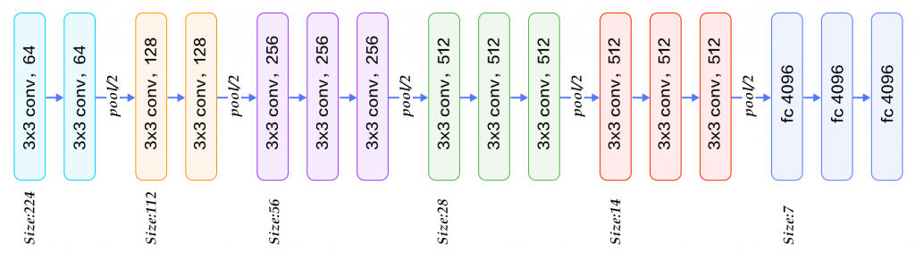
그림. VGG-16 네트워크 구성
slim.arg_scope()를 이용하여 VGG-16 네트워크 정의를 간단히 사용할 수 있다.
1 2 3 4 5 6''' # 네트워크 모델 로드: VGG-16 ''' vgg = tf.contrib.slim.nets.vgg with slim.arg_scope(vgg.vgg_arg_scope()): logits, end_points = vgg.vgg_16(inputs=images, num_classes=120, is_training=True)
체크포인트로부터 파라미터 초기화하기
네트워크 정의를 가져왔다면, 이미지넷 데이터로 학습된 체크포인트를 이용하여 네트워크 파라미터를 초기화한다. 문제는 이미지넷의 경우 출력 레이어가 1000개로 구성되는 반면, 품종 분류에서는 출력 레이어가 120개로 구성된다. 따라서 마지막 출력 레이어는 체크포인트로부터 파라미터를 초기화할 수 없다. 이처럼 대개의 경우 전체 네트워크의 마지막 full connected 레이어는 학습하려는 문제에 의존적이므로 체크포인트로부터 파라미터를 복원하는 것이 의미가 없다. 반면 이미지의 feature map을 추출할 수 있는 컨볼루션 필터의 경우 이미지 유형에 따라 달라지지만 많은 부분을 공유하게 된다. 따라서 이미지넷 데이터셋으로부터 학습된 체크포인트에서 VGG-16 네트워크의 앞의 컨볼루션 레이어 영역의 파라미터만 복원하는 방식으로 초기화한다.
먼저 pre-trained된 체크포인트 파일을 다운로드한다. 대표적인 이미지 네트워크 모델에 대한 정의와 체크포인트에 대한 내용은 TensorFlow-Slim image classification library에서 확인할 수 있다.
1 2 3 4 5 6 7 8 9 10 11''' # 체크포인트로부터 파라미터 복원하기 ''' # 다운로드한 VGG-16 체크포인트 파일 경로 model_path = '/home/itrocks/Backup/Model/TF-Slim/vgg_16.ckpt' # 마지막 fc8 레이어는 파라미터 복원에서 제외 exculde = ['vgg_16/fc8'] variables_to_restore = slim.get_variables_to_restore(exclude=exculde) saver = tf.train.Saver(variables_to_restore) with tf.Session() as sess: saver.restore(sess, model_path)
또는 tf.contrib.framework.assign_from_checkpoint_fn(...) 함수를 이용하여 초기화 함수만을 정의한 후, slim.learning.train(...) 함수로 학습 진행시 인자로 전달할 수 있다.
1 2 3 4 5 6 7 8 9 10init_fn = tf.contrib.framework.assign_from_checkpoint_fn(model_path, variables_to_restore, ignore_missing_vars=True) ... # 훈련하기 final_loss = slim.learning.train(train_op=train_op, logdir=logdir, init_fn=init_fn, number_of_steps=500000, summary_op=summary_op, save_summaries_secs=300, save_interval_secs=600)
exclude할 레이어는 레이어 이름으로 설정할 수 있다. TF-Slim에서 제공하는 VGG-16 네트워크 정의는 vgg.py에서 확인할 수 있으며, 이 중 마지막 레이어에 대한 정의는 다음과 같다.
1 2 3 4 5 6 7 8 9def vgg_16(...): ... with tf.variable_scope(scope, 'vgg_16', [inputs]) as sc: ... net = slim.conv2d(net, num_classes, [1, 1], activation_fn=None, normalizer_fn=None, scope='fc8') ...
따라서 마지막 레이어인 'vgg_16/fc8'을 exclude 항목에 지정하도록 한다.
Fine-Tuning하기
훈련할 네트워크를 복원했다면, 이후의 과정은 아래와 같이 기본 학습과정과 동일하다.
- 손실함수 정의
- 옵티마이저 정의
- 메트릭 정의
- 훈련하기
손실함수 정의
1 2loss = slim.losses.softmax_cross_entropy(logits=logits, onehot_labels=labels) total_loss = slim.losses.get_total_loss()
옵티마이저 정의
adam 옵티마이저를 정의하며, learning rate decay를 적용한다.
1 2 3 4 5 6 7 8 9 10 11 12 13 14 15 16 17''' # 옵티마이저 정의: Adam # learrning rate decay 적용 ''' initial_learning_rate = 0.0002 learning_rate_decay_factor = 0.9 num_epochs_before_decay = 2 global_step = get_or_create_global_step() num_batches_per_epoch = num_samples / batch_size num_steps_per_epoch = num_batches_per_epoch # Because one step is one batch processed decay_steps = int(num_epochs_before_decay * num_steps_per_epoch) lr = tf.train.exponential_decay(learning_rate=initial_learning_rate, global_step=global_step, decay_steps=decay_steps, decay_rate=learning_rate_decay_factor, staircase=True) optimizer = tf.train.AdamOptimizer(learning_rate=lr)
메트릭 정의
1 2 3 4 5 6 7predictions = tf.argmax(logits, 1) targets = tf.argmax(labels, 1) correct_prediction = tf.equal(predictions, targets) accuracy = tf.reduce_mean(tf.cast(correct_prediction, tf.float32)) tf.summary.scalar('losses/Total', total_loss) tf.summary.scalar('accuracy', accuracy) summary_op = tf.summary.merge_all()
훈련하기
1 2 3 4 5 6 7 8 9 10 11 12 13 14# logging 경로 설정 logdir = '/home/itrocks/Downloads/dog_model/' if not tf.gfile.Exists(logdir): tf.gfile.MakeDirs(logdir) # 훈련 오퍼레이션 정의 train_op = slim.learning.create_train_op(total_loss, optimizer) final_loss = slim.learning.train(train_op=train_op, logdir=logdir, init_fn=init_fn, number_of_steps=500000, summary_op=summary_op, save_summaries_secs=300, save_interval_secs=600) print('Finished training. Final batch loss %f' %final_loss)
훈련이 실행되면 텐서보드를 실행하여 훈련 과정을 모니터링한다.
1$ tensorboard --logdir=./dog_model
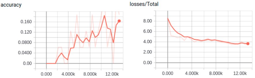
그림. 텐서보드로 개 품종 분류 훈련 모니터링
평가하기
평가하는 과정은 MNIST와 완전히 동일하다.
1 2 3 4 5 6 7 8 9 10 11 12 13 14 15 16 17 18 19 20 21 22 23 24 25 26 27 28 29 30 31 32 33 34 35 36 37 38 39 40 41 42 43 44 45 46 47 48 49 50tf.logging.set_verbosity(tf.logging.INFO) ''' # 평가 데이터 로드 ''' batch_size = 16 tfrecord_dataset = tf_record_dataset.TFRecordDataset( tfrecord_dir='/home/itrocks/Git/Tensorflow/dog-breed-classification.tf/raw_data/dog/tfrecord', dataset_name='dog', num_classes=120) # Selects the 'train' dataset. dataset = tfrecord_dataset.get_split(split_name='validation') images, labels, num_samples = load_batch(dataset, batch_size=batch_size, height=224, width=224) ''' # 네트워크 모델 로드: VGG-16 ''' vgg = tf.contrib.slim.nets.vgg with slim.arg_scope(vgg.vgg_arg_scope()): logits, end_points = vgg.vgg_16(inputs=images, num_classes=120, is_training=True) ''' # 메트릭 정의 ''' logits = tf.argmax(logits, 1) labels = tf.argmax(labels, 1) # Define the metrics: names_to_values, names_to_updates = slim.metrics.aggregate_metric_map({ 'eval/Accuracy': slim.metrics.streaming_accuracy(logits, labels), #'eval/Recall@5': slim.metrics.streaming_recall_at_k(logits, labels, 5), }) ''' # 평가하기 ''' # logging 경로 설정 log_dir = '/home/itrocks/Downloads/dog_model/' eval_dir = '/home/itrocks/Downloads/dog_model-eval/' if not tf.gfile.Exists(eval_dir): tf.gfile.MakeDirs(eval_dir) if not tf.gfile.Exists(log_dir): raise Exception("trained check point does not exist at %s " % log_dir) else: checkpoint_path = tf.train.latest_checkpoint(log_dir) metric_values = slim.evaluation.evaluate_once( master='', checkpoint_path=checkpoint_path, logdir=eval_dir, num_evals=100, eval_op=names_to_updates.values(), final_op=names_to_values.values()) names_to_values = dict(zip(names_to_values.keys(), metric_values)) for name in names_to_values: print('%s: %f' % (name, names_to_values[name]))
학습이 완전히 완료하려면 이틀정도 걸릴 것으로 보이는데, 시간이 없는 관계로 생략한다 like a Fermat.
참고자료
- TensorFlow-Slim
- TensorFlow-Slim image classification library
- TF-Slim Walkthrough
- TensorFlow > Programmer's Guide > Variables: Creation, Initialization, Saving, and Loading
- Difference between variable_scope and name_scope in TensorFlow
- 텐서플로우(TensorFlow) 시작하기
- Kaggle > MNIST as .jpg
- Daniil's blog > Tfrecords Guide
- Standford Dogs Dataset
- tf-slim-tutorial
- dog-breed-classification.tf
- TRANSFER LEARNING IN TENSORFLOW USING A PRE-TRAINED INCEPTION-RESNET-V2 MODEL